Priors

A prior says two things about a parameter: where it may be, and how likely each value in that range is. In GalSpec it is set on the parameter itself – the attribute astropy already reserves for the user’s fitter – so the prior sits next to the thing it describes instead of in a dictionary passed to the sampler at call time:

model.sigma_w0.prior = priors.Uniform(300.0, 8000.0)

This page covers the shapes that exist, what the fitter does with them, and three worked examples taken from example/: the published recipe, a prior centred on another parameter, and a prior that can switch a component off entirely. For the fit those priors belong to, see Example: fitting a strong AGN.

The four shapes

from galspec import priors

model.amplitude.prior = priors.LogUniform(1e-3, 30.0)   # flat per decade
model.sigma_c.prior   = priors.Uniform(300.0, 8000.0)   # flat in the value
model.amp_w0.prior    = priors.Uniform(0.0, 1.0)        # a ratio: bounded
model.amp_w1.prior    = priors.SpikeAndSlab(p_off=0.5)  # may be exactly zero

# a prior that names another parameter: broad H-beta's wind shift is centred on
# broad H-alpha's, with 5% of H-alpha's wind width as its sigma and five of those
# widths as a hard limit
model.set_prior("b_hbeta.dv_w0",
                priors.Normal(mean="b_halpha.dv_w0", sigma=0.05,
                              scale_from="b_halpha.sigma_w0", nsigma=5))

shape	use it when	in the published recipe
Uniform(lower, upper)	the range is already the physical one	every width, shift and ratio; the continuum power-law index
LogUniform(lower, upper)	the parameter spans decades	every line peak, and the iron amplitude: from invisible to three times the brightest pixel
Normal(...)	the value is expected near a number, or near another parameter	the soft tie (below)
SpikeAndSlab(p_off)	the parameter may be absent, not merely small	the wing gate in the component-count run (below)

A parameter whose prior is never mentioned is uniform over its default bounds, and the examples refuse to start in that state – a stray parameter then samples its whole box and the run looks fine while it happens.

A centred prior, in detail

priors.Normal returns a galspec.CenteredPrior; mean is a number or the name of another parameter. The width of the Gaussian can be written three ways:

• absolute (default): sigma is in the parameter’s own units;

• relative=True: sigma is a fraction of the centre’s value, so the prior widens with the profile it is centred on;

• scale_from="name": sigma is a fraction of that parameter’s value – how a shift is constrained in units of a line width.

log=True makes it multiplicative (a log-normal), the right shape for an amplitude; it cannot be combined with relative, because in log space sigma is already a fraction.

nsigma is a hard limit, not a suggestion: beyond it the prior is exactly zero. The default is seven, where 1.3e-12 of the Gaussian’s mass is left and float64 can no longer tell a cumulative probability from 1. The prior is truncated to the parameter’s own box intersected with that range, so when the box is narrower, the box wins. A posterior that piles up against a hard limit is then a bound on the parameter, not a measurement of it – which is why the tied example reports how much of the posterior sits there.

What the fitter does with them

A prior is a transform of the unit cube. The sampler draws u in [0, 1] and the prior maps it one-to-one onto the parameter’s range, carrying the Jacobian inside the transform. Because the map is a bijection and not a sampling density, the number the run reports is the evidence of the stated prior – nested sampling’s prior volume stays meaningful.

Dependencies are resolved, not assumed. A prior that names another parameter must be drawn after it. galspec.resolve_prior_dependencies() resolves names (flat, then qualified, then a unique bare match – an ambiguous one is an error rather than a guess), rejects cycles, and returns an order in which independent parameters keep their original position, so a model without centred priors transforms exactly as it did before. Both fitters walk that order, and tests/test_priors_tied.py asserts they agree to 1e-9.

Log-scaled parameters are truncated in log space. An amplitude’s box is stored in log10 units, so the truncation range is exponentiated before it reaches the prior; the fitters do that, or a tie silently lands in the wrong place.

The published recipe

set_priors in example/iras07546_model.py, condensed:

what	range	why that shape
line peaks	1e-3 to 3x the brightest pixel, log-uniform	four decades, from invisible to implausibly strong
wind / core ratio	0-1, uniform	no wind is brighter than its own core
narrow shift	+-1000 km/s, uniform	one shift shared by every narrow line, measured from [O III]. There is no narrow width to give a prior to: it is in the measured template, which is what makes the narrow lines one number each instead of three.
[S II] 6716/6731 ratio	both peaks log-uniform, free	it is a density diagnostic, not an atomic constant – unlike [O III], [N II] and [O I], whose ratios are tied
broad shifts	core +-2 500, wind +-6 000 km/s, uniform	a core within a few widths of rest, a wind free to be offset by more
broad core and wind	300-8000 km/s, uniform	one box for both: a wing is not assumed broader than its core, and a 25 000 km/s ceiling only puts prior where the data are not
continuum level	0.2-4x the line-free windows, log-uniform	cannot be negative, cannot swamp the lines
Fe II amplitude	1e-3 to 3x the continuum level	the only free iron parameter

Worked example: a prior centred on another parameter

The three Balmer lines come from the same gas, so the published fit ties broad H-beta’s and H-gamma’s shifts and widths to broad H-alpha’s. A tie is an absolute statement: the tied parameter cannot disagree, so the fit cannot report whether the tie was right, and a real difference would be absorbed silently by the amplitudes.

The alternative is not to free all eight parameters – the difference between two widths is then dominated by whatever the data cannot constrain. What is wanted is “near H-alpha’s value, and not farther than this”:

# a width: 20% of H-alpha's width, at most five widths away
model.set_prior("b_hbeta.sigma_c",
                priors.Normal(mean="b_halpha.sigma_c", relative=0.20, nsigma=5))
# a shift: 5% of that component's H-alpha *width* (not of the shift, which can be
# near zero), used as the standard deviation
model.set_prior("b_hbeta.dv_c",
                priors.Normal(mean="b_halpha.dv_c", sigma=0.05,
                              scale_from="b_halpha.sigma_c", nsigma=5))

That is the whole construction, and example/fit_iras07546_jax_tied.py is the worked fit with it applied: 35 free parameters instead of 27, with WIDTH_FRACTION = 0.20, SHIFT_FRACTION = 0.05, MAX_SIGMA = 5.0 and CAP_TOLERANCE (when a pull counts as sitting on the limit) as named constants at the top of the file.

The number to read is the pull – the difference from H-alpha’s value in units of the tie width. A pull of zero means the data agree with the tie; a pull of one means the difference is as large as the prior allowed for; a pull of five or more means the data asked for more than the prior permits, and the fitted value is a compromise rather than the likelihood’s own answer.

The evidence moves too, and its sign has to be read carefully. For a Gaussian of width \(\sigma_{\rm tie}\) against a posterior of width \(\sigma_{\rm post}\), each released parameter costs

\[\Delta \ln Z \;\approx\; \ln \frac{\sigma_{\rm tie}\sqrt{2\pi}}{\sigma_{\rm post}} ,\]

which for the eight parameters is +21.5 if the tie is right (the script computes it from each parameter’s own posterior width). A drop of that size is the expected cost of a freedom the data did not need; a rise means the likelihood gained more than the prior volume cost, i.e. the tie was wrong.

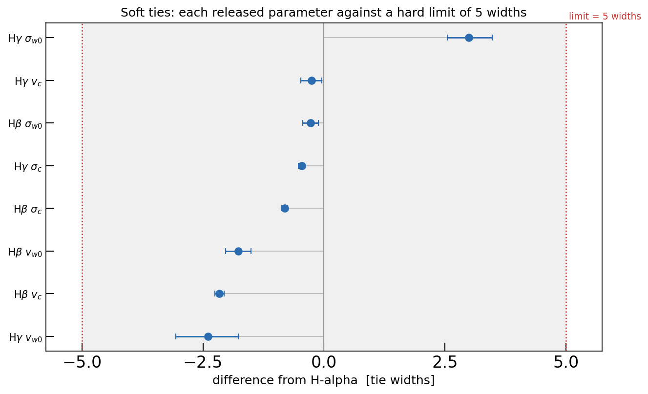
Each released parameter against H-alpha, in tie widths. The shaded band is where the prior allows the difference, the red lines its hard limit at five tie widths, and every point lies inside both.

On IRAS 07546+3928 the answer is measured, and it is not the answer the previous generation of this page gave – which is the useful part. The eight released parameters (H-beta and H-gamma, core and wind, width and shift) split three ways:

parameter	H-alpha	line	difference	fractional	pull
b_hbeta.sigma_c	1 227.6	1 029.4	-198.2	-16.1%	-0.81
b_hbeta.dv_c	234.8	102.2	-132.7	-56.5%	-2.16
b_hbeta.sigma_w0	4 214.2	3 978.2	-235.4	-5.6%	-0.28
b_hbeta.dv_w0	-398.4	-770.5	-372.6	-93.5%	-1.77
b_hgamma.sigma_c	1 227.6	1 114.6	-112.8	-9.2%	-0.46
b_hgamma.dv_c	234.8	218.9	-15.9	-6.8%	-0.26
b_hgamma.sigma_w0	4 214.2	6 732.7	+2 522.9	+59.9%	+2.99
b_hgamma.dv_w0	-398.4	-903.2	-504.3	-126.6%	-2.39

The four core parameters agree with H-alpha’s – pulls inside 0.9 for the widths and 2.2 for the shifts – so for the narrow cores the hard tie was right and could have stayed. The four wind parameters are where the two lines differ: H-beta’s wind is H-alpha’s within a third of a tie width in width and 1.8 in shift, but H-gamma’s is 60% broader and 504 km/s bluer, at +2.99 of its five-width window.

The soft fit comes out +833.21 +- 0.71 above the hard tie: the eight parameters bought about 863 nats of likelihood (chi2/dof 0.315 -> 0.285 over 56 921 degrees of freedom) and cost 21.2 in prior volume. 863 - 21.2 = 842 against the measured 833, which agrees to the accuracy of a chi2/dof printed to three digits (0.001 of it is 57 nats). The evidence went into the likelihood, not into book-keeping.

Two things about that number are worth stating plainly, because it is larger than the pulls suggest and it is the kind of result that gets over-read:

• A 3.0-sigma pull plus an 833-nat evidence gain is not a contradiction. The pulls are per parameter and are measured relative to H-alpha’s value; the evidence is the joint likelihood gain from re-shaping three line profiles at once, and a change of a few per cent in a broad wing that spans 1 500 A moves a lot of pixels. The eight parameters are also correlated – H-beta’s shifted wind and H-alpha’s width trade against each other – so no single pull carries the gain.

• Nothing here sits against a hard limit. In the earlier version of this page the two wind widths piled up on the 8 000 km/s ceiling of the width prior, which is a prior artefact and not a measurement; with the narrow lines described by the measured [O III] template (see Example: fitting a strong AGN) the released widths come out at 3 978 +- 94 and 6 733 +- 330 km/s, both inside the box, with none of their posterior against either wall. The released parameters are therefore measurements, which they were not before.

H-alpha’s own numbers move a little when the ties are released, and the size of that move is the honest error bar on the tie assumption:

parameter	hard tie	soft tie	difference
b_halpha.sigma_c	1 194 +- 6	1 228 +- 8	34 (3 sigma)
b_halpha.sigma_w0	4 316 +- 41	4 214 +- 61	102 (2 sigma)

Three per cent, and the shifts move by less (234.8 against 209.4). So the answer is not sensitive to whether the tie holds – what is sensitive is the evidence, and that is the quantity the tie was deciding.

A gain that size is worth checking against the sampler before it is quoted, and the control is cheap. JNesty seeds its live points from a fixed key, so a rerun visits the same live points – but bitwise identity is not what comes back: two runs of this fit on the same GPU differed by 0.45 nats, which is inside the error bar, from the last bits of a GPU sum feeding the sampler’s ordering. The 27-parameter fit repeats to about the same tolerance (three runs span 1.8 nats). What also matters is the live-point count: rerunning the hard-tie fit at 1 000 points instead of 400 moved it by 2 nats with the same posteriors. So the honest error on a single evidence is a few nats rather than the 0.6 the run reports – and this difference is larger by two orders of magnitude. The soft fit runs at 1 000 live points, which is why its error bar (0.40) is smaller than the hard fit’s (0.58) despite having eight more parameters.

Two caveats belong with the numbers above:

• The tie width is a physical statement, and it is the choice that decides the answer. 20% of the width says the two profiles move like the same gas to within a fifth; a galaxy whose H-beta region really were twice as broad as its H-alpha region would show pulls of ~5 and would be reported as such, not smoothed away.

• Component *i* is tied to component *i*. With one wind per line the pairing is unambiguous; with more it is a choice, and the example pairs them in order.

Worked example: switching a component off

How many broad components does a profile need? The alternative to fitting k and comparing evidences is to let the sampler decide: give the line k components and let every component after the first carry a toggle prior – with some probability its amplitude is exactly zero.

Nothing special is needed in the models: Line_MultiGauss(n_components=k) is a core plus k - 1 wings, each with its own amplitude ratio, shift and width.

# a spike at exactly zero (probability 0.2), else a linear slab on (0, 1]
for name in ("b_halpha", "b_hbeta", "b_hgamma"):
    model.set_prior(f"{name}.amp_w0", priors.SpikeAndSlab(p_off=0.2, lower=0.0,
                                                         upper=1.0))

The zero is exact, not small. That is what makes it work: a point mass has finite prior volume – p_off of the cube – while a density on the reals has none. A nested sampler can find a region of finite volume; it could never find a point of measure zero. The Bayes factor of the component follows from the prior odds it was given:

\[\mathrm{BF} = \frac{P(\text{on})/P(\text{off})}{(1 - p_{\rm off})/p_{\rm off}} .\]

Dividing the prior odds out matters: with a ladder of p_off the higher components are a priori unlikely and would otherwise look rejected for that reason alone.

A component that is switched off is unambiguous. One that is barely on is not: at 1% noise an unneeded Gaussian can sit at 1% of the core peak and buy a little chi-square from the noise, with a Bayes factor of ~400 in favour. So the count is defined with a floor – 3% of the core peak in the example – and the fit still puts posterior mass between zero and the floor. The floor is part of the definition of “needed”, not a hidden prior.

The recipe, as example/fit_iras07546_jax_toggle.py applies it:

• only the three Balmer lines get four components; He I and He II keep one broad Gaussian, and the Fe II kernel follows broad H-alpha. 37 free parameters – six fewer than the Gaussian narrow-line version of this fit, because the narrow lines are one measured profile with one shift (example/iras07546_model.py);

• one width prior for everything, 300-8000 km/s, the same box as the published fit – a wing is not required to be broader than the core;

• a ladder p_off = 0.2, 0.5, 0.7. The likelihood cannot tell two wings apart (exchanging them leaves the spectrum bit-identical), so the prior is the only place an asymmetry can live;

• decide by the mode of the floored count, then refit at that k with plain priors if an evidence is wanted.

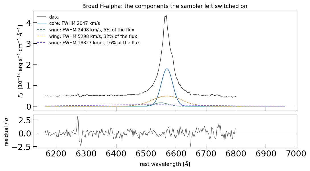
The four components the run reports for broad H-alpha, sorted by width.

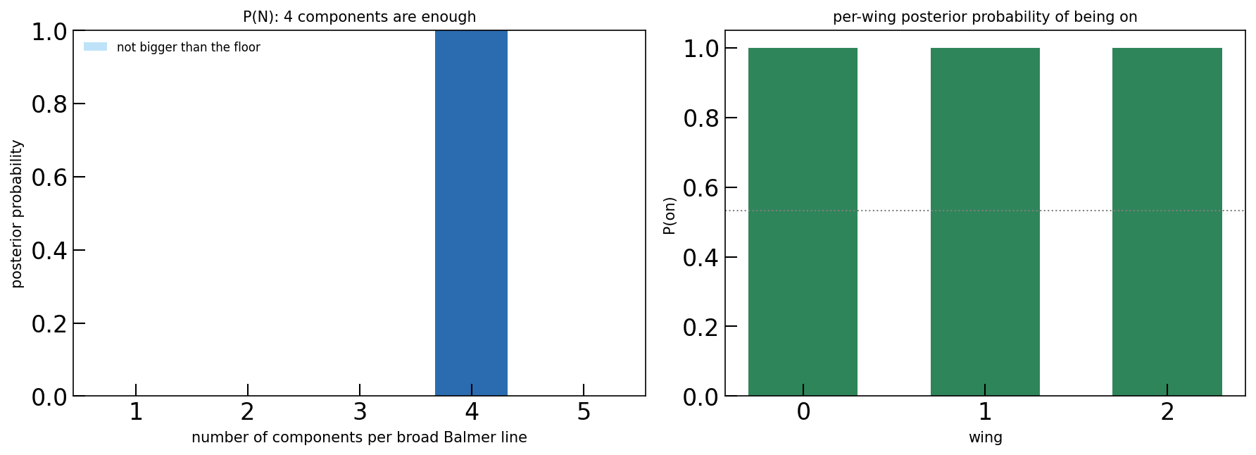
Where the count comes from: left, the posterior on how many components the profile needs (1.000 for four); right, the probability that each of the three wings is on.

The answer on IRAS 07546+3928: the run asked for at most four broad components and returned four – a core plus three wings. All 211 675 equally weighted samples have all three wings on and all three above the 3% floor, so P(3 wings) = 1.000 and every Bayes factor is unbounded above: with the narrow lines described by the measured template rather than a Gaussian each, the count is not a marginal call at all. (The same model with Gaussian narrow lines returned 0.84 here, so the pixels that voted against the widest wing were being used to pay for the narrow-line mismatch.) Sorted by width, broad H-alpha comes out as:

component	peak / core peak	FWHM [km/s]	dv [km/s]	share of the broad flux
core	1.000	2 047	+312	47.0%
wing 1	0.091	2 498	-908	5.1%
wing 2	0.272	5 298	+12	32.5%
wing 3	0.038	18 827	-3 590	16.2%

Two caveats come with that answer. The pedestal (wing 3) sits on the width ceiling – 18 827 km/s of FWHM is 7 995 km/s of sigma against the 8 000 km/s bound – so how wide it is, and possibly how many components describe the base of the line, is limited by the adopted range rather than by the data. And the count is floor-sensitive in the expected way: the pedestal peaks at 3.8% of the core, just above the 3% floor, so at a 5% floor the count is three and at 10% it is two – not because the pedestal is noise (its Bayes factor is unbounded) but because a coarser floor is a different definition of “a component”.

Calibration on mocks with known answers (develop/dev_jax/broad_line_components.py, four mocks of 1, 2, 3 and 4 components at 1% noise; develop/ is a separate, local-only repository, so the name is a pointer and not a link) says three things. The count is the minimum the data need, not the number that generated them: it is exact for the 1-, 2- and 3-component mocks, and 3 for the 4-component one, because three overlapping wings that differ only in width are not separately required by 1%-noise data. The linear slab is the right one – a log slab puts a spurious wing above the floor in a third of the posterior on the 2-component mock by concentrating density where an extra Gaussian hides in the noise. And use 1000 live points when the count is the answer: 400 gets that same mock wrong, reproducibly.

What it does not do:

• it does not make an extra Gaussian expensive – the prior says a component is unlikely a priori, and with 1% noise the likelihood sometimes still prefers one. The floor is what turns a continuum of small amplitudes into a decision;

• it does not identify which component is which, or order them;

• its evidence is not an evidence for a k-component model: a toggled model is a mixture over subsets, so quote the count from the gated run and refit at that count for an evidence ratio.

The statistics is standard – a spike-and-slab prior for variable selection goes back to George & McCulloch (1993) and Kuo & Mallick (1998). Trans-dimensional sampling (Green 1995; diffusive nested sampling, Brewer 2014) is the more general route and needs no floor, but it changes the parameter count from sample to sample, which defeats the fixed-size vectors that jit/vmap batching needs. The variant here needs no change to the sampler at all.

Saving priors with a fit

A saved fit carries its priors: each is stored as its type plus its constructor arguments, together with the name of any parameter it is centred on, so the file is enough to rebuild the prior transform and resume the sampler. The one exception is a prior supplied as a bare Python function – that has no data form, so the loader warns and keeps only the resolved bounds.