
Example: fitting a strong AGN#
One AGN spectrum, one model, one sampler, and the step before it: measuring the narrow
lines’ profile. Every code block on this page is a cell of
example/fit_iras07546_jax.ipynb – the notebook builds the model literally, seventeen
constructors and then the ties, with no build_model() in the way – so a block can be
copied into a notebook and run:
example/fit_iras07546_jax.ipynb– the whole fit, cell by cell: the data, the model, the ties, the priors, the sampler, the figures;example/fit_iras07546_o3_template.py– step 2, measures the narrow-line profile on the [O III] doublet and writes it to a file (the code calls this stage 1: it is the first of the two fits);example/iras07546_model.py– the same model as an importable module, for the three example scripts.tests/test_example_notebook.pyexecutes the notebook’s model cells and compares them with the module’s, tie for tie and prior for prior, so the two copies cannot drift apart.
IRAS 07546+3928 at z = 0.0953: 4200-6800 A in the rest frame, 57 000 pixels at 0.046 A
sampling, H-gamma through H-alpha with the strong forbidden lines. The fit has 27 free
parameters, runs with 400 live points and dlogz = 0.01, and takes about eight minutes
on one GPU. It is the first of two examples: the other, Example: measure the black hole and the host galaxy,
fits a low-luminosity AGN whose continuum is starlight instead of a power law.
Twelve of those 27 are narrow-line parameters – eleven peak amplitudes and one shared
velocity shift; the narrow profile is not fitted at all. It is one measured object,
example/data/iras07546_narrow_template.txt, extracted from the [O III] doublet in
step 2 and shared by all ten narrow lines. That is what makes the parameter count 27
instead of 30, and step 2 is where the shape comes from, so it comes first.
The spectrum#
Start with the data as it arrives, before anything is cut. IRAS 07546+3928 was observed with a long slit and a grism, so the flux is a FITS primary array with a start wavelength and a step in the header, and no error array: the error has to come from the spectrum itself.
The figure shows the observed flux, the same flux with the foreground reddening removed,
and the +-1 sigma band that the fit will be given. Two things are worth reading off it.
The correction is a slope, not a rescale – E(B-V) = 0.176 is a modest Galactic
extinction, so it changes the continuum shape and leaves the lines where they are. And the
error is not noise on a smooth curve: it grows with the flux, because part of it is the
photon noise of the source itself.
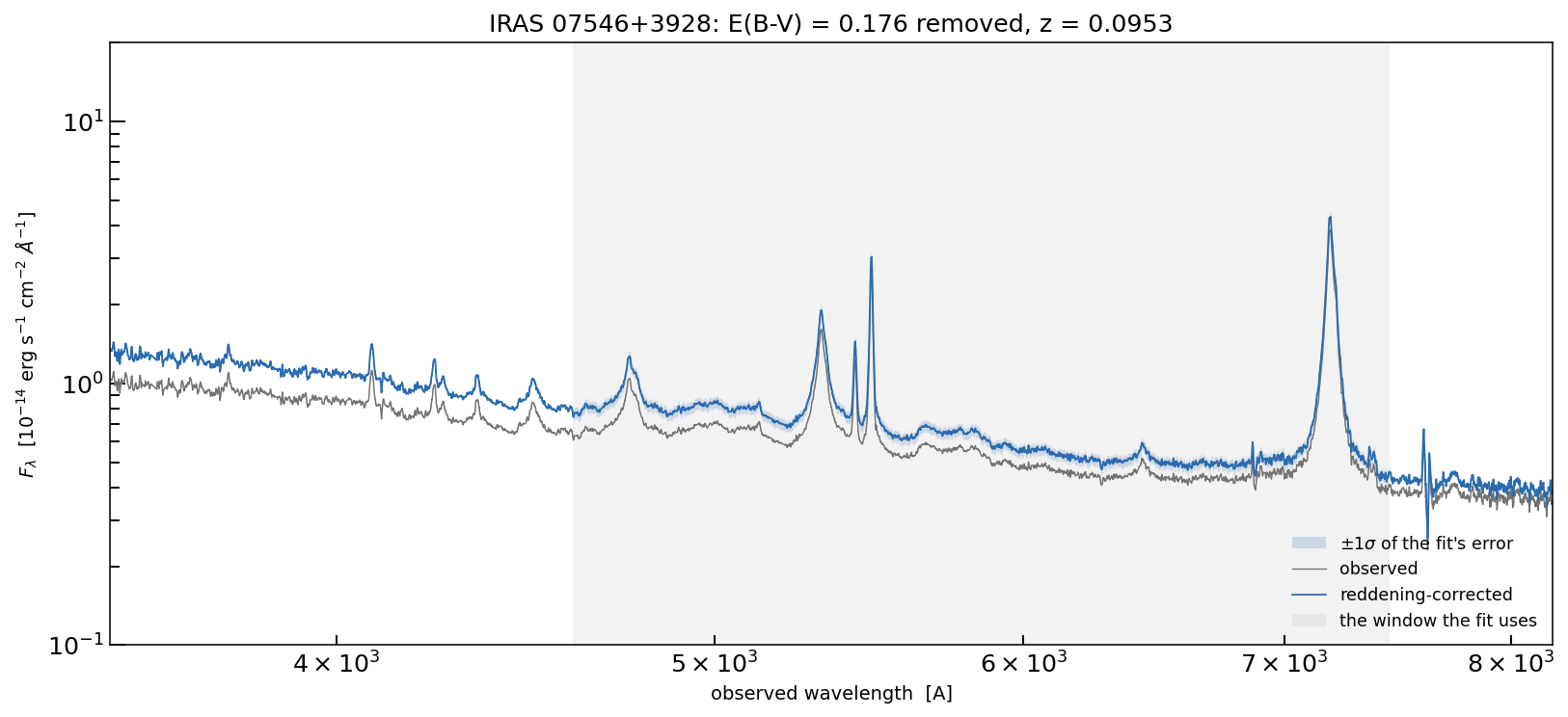
The observed spectrum (grey), the same after the Milky Way reddening is removed (blue), and +-1 sigma of the error the fit is given (band). The shaded region is the wavelength range the fit actually uses – and it is the only range the error exists over, because that is where it is measured (section 1).#
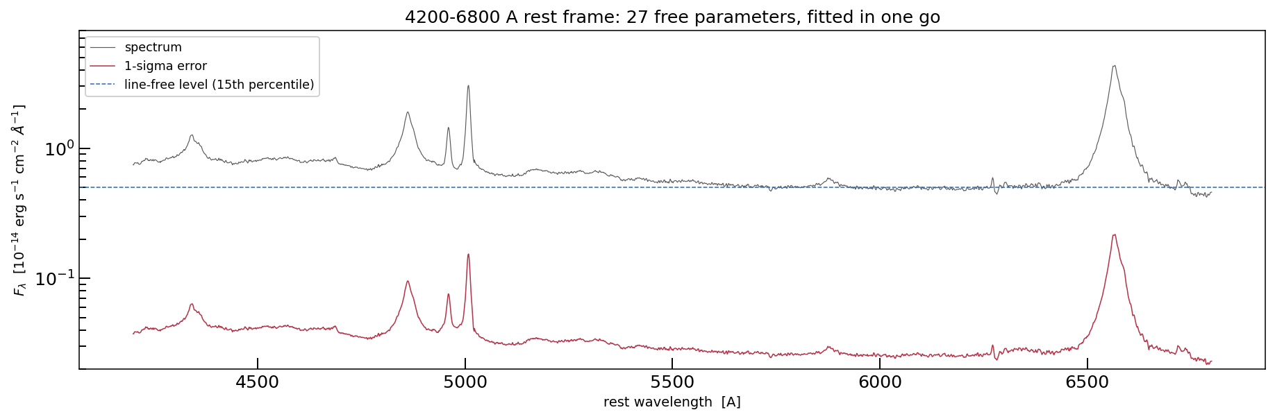
The fitted window, 4200-6800 A rest frame: the spectrum, the error on its own scale (it rises where the spectrum does, because part of it is photon noise), and the line-free level the priors are scaled from – the 15th percentile of the flux. The scale is logarithmic so that a 2% error and a fourfold line peak fit in one panel.#
1. Read the spectrum#
Three transformations happen in one cell: the reddening correction (divide by the dust
transmission on the observed grid, i.e. multiply by 10**(0.4 A_lambda), with the CCM89
law and E(B-V) = 0.176 – dust in our own Galaxy, not at the redshift of the object),
the shift to the rest frame
(wave / (1 + z)), and the window. The error is re-derived from the scatter of the
spectrum rather than trusted from a header: subtract a running median, take the median of
the absolute remainder in the same window – which ignores the few pixels that belong to
emission lines – divide by 0.6745 to turn it into a Gaussian sigma, and smooth over a few
hundred A. Then add PHOTON_FRACTION of the flux in quadrature: the photon noise of the
source, plus what the model does not describe exactly (flux calibration, the shape of the
Fe II template, departures from a pure power law).
That last step matters more than it looks, in two ways. A wrong error scale does not
make a fit fail; it makes every posterior too narrow or too wide by the same factor,
invisibly – the parameter is 5% here, and it is the one number in the data step that is a
judgement. And the order of the operations is part of the model: the recipe reads
neighbouring pixels, so measuring it before the wavelength cut instead of after moves the
4 000 pixels at the window edges by up to 8%, which is tens of nats of evidence for a
spectrum that looks identical. The cell derives the error from the window, and
tests/test_example_notebook.py asserts that this cell returns the same three arrays as
load_spectrum() in example/iras07546_model.py – bit for bit, not approximately.
# %% data
from astropy.io import fits
from extinction import ccm89, remove

with fits.open(DATA_FILE) as hdul:
    header = hdul[0].header
    flux_obs = np.asarray(hdul[0].data, dtype=float) * 1e14     # 1e-14 erg/s/cm2/A
wave_obs = header["CRVAL1"] + header["CD1_1"] * np.arange(flux_obs.size)

# 1. foreground reddening: our own Galaxy, A_V from NED, CCM89
flux_dred = remove(ccm89(wave_obs, E_BV, r_v=3.1, unit="aa"), flux_obs)

# 2. rest frame, then the window the fit uses
wave_rst = wave_obs / (1.0 + REDSHIFT)
use = (wave_rst > WAVE_MIN) & (wave_rst < WAVE_MAX)
wave, flux = wave_rst[use], flux_dred[use]
wave_window_obs = wave_obs[use]            # the same window, in the observed frame

# 3. the error, measured from the window (the file has none).  The order matters: the
#    recipe reads the neighbouring pixels, so measuring it after the cut -- and not on
#    the whole spectrum -- is what makes these the arrays the example scripts fit.
window = 751                                         # ~34 A: wider than any line core
baseline = median_filter(flux, size=window, mode="nearest")
scatter = median_filter(np.abs(flux - baseline), size=window, mode="nearest") / 0.6745
scatter = median_filter(scatter, size=4 * window + 1, mode="nearest")
statistical = np.maximum(scatter, ERROR_FRACTION * np.abs(flux))
error = np.hypot(statistical, PHOTON_FRACTION * np.abs(flux))

print(f"data: {wave.size:,} pixels, {wave[0]:.0f}-{wave[-1]:.0f} A (rest frame)")
print(f"      peak flux {flux.max():.2f}, line-free level {np.percentile(flux, 15):.2f}"
      f"  [1e-14 erg/s/cm2/A]")
2. Measure the narrow-line profile on [O III]#
A narrow emission line in an AGN is not a Gaussian. It is the virial and turbulent kinematics of a whole region, and its profile has wings that a Gaussian cannot bend into. Fitting a Gaussian per line therefore does two bad things at once: it spends a free width per line on a shape the data constrain much better once, and the widths it returns depend on which lines are bundled together.
The alternative is to measure the shape once, on the line with the most signal per pixel, and give it to the rest with an amplitude each. [O III] 5007 is that line here: narrow, strong, and sitting in a window where the continuum is smooth and close by.
Two decisions make the measurement a measurement rather than a choice:
A local fit, not a global one. The window is 160 A, 3 505 pixels. The broad H-beta wing runs underneath it and would otherwise be free to reshape the narrow profile – which is exactly the degeneracy that a global fit cannot avoid.
The iron stays in. [O III] 5007 sits where the Fe II pseudo-continuum is still strong – the published fit gives it an amplitude of 0.25, and the local fit below starts there. Leave it out and the window fit has nowhere to put that flux but a very broad wing on [O III] itself, which then goes into the template and is added under every narrow line.
The window’s model is three objects: a degree-3 polynomial on an abscissa mapped onto
[-1, 1], the iron template, and a three-component Line_MultiGauss_doublet – a core
plus two winds. Three components is not assumed: it is what the evidence chose between
two and three (the scan that did that is develop/dev_template/stage1_o3_template.py,
a local script that is not part of this repository; what is in this repository is the
run that produces the template). The wing width is capped at 1 500 km/s, because a
broader component is indistinguishable from the continuum over this window and will
absorb it if allowed to.
def build_window_model(n_components=N_COMPONENTS, degree=POLY_DEGREE, window=WINDOW):
    """Polynomial continuum + Fe II + an [O III] doublet of ``n_components`` Gaussians.

    Initial values are the published global fit's, so the sampler starts where the
    spectrum is known to be; they are values, not an answer -- the window is fitted
    from scratch and its priors are below.
    """
    continuum = jxm.Polynomial1D(degree=degree, domain=tuple(window),
                                 window=POLY_WINDOW, name="Cont")
    continuum.label = f"Continuum (degree {degree})"
    o3 = jxm.Line_MultiGauss_doublet(
        n_components=n_components,
        amp_c0=1.9, amp_c1=1.9 / O3_RATIO, dv_c=50.0, sigma_c=280.0,
        wavec0=LINE_WAVE["OIII_5007"], wavec1=LINE_WAVE["OIII_4959"],
        name="OIII",
        par_w={f"{stem}_w{i}": value
               for i in range(n_components - 1)
               for stem, value in (("amp", 0.09), ("dv", -200.0), ("sigma", 900.0))})
    # the 5007/4959 ratio is atomic: tied, not fitted
    o3.amp_c1.tied = jxm.tie.tie_MultiGauss_doublet_ratio("OIII", O3_RATIO)

    # amplitude and width are fitted; a velocity shift is not, because across 160 A
    # it is degenerate with the shape of the continuum
    iron = jxm.IronTemplate(amplitude=0.25, sigma=1200.0, z=0.0,
                            template_name="park2022", sigma_max=IRON_SIGMA_MAX,
                            name="FeII", fixed={"z": True, "dv": True})
    iron.label = "Fe II"
    o3.label = "[O III]"
    return continuum + iron + o3


def set_window_priors(model, flux):
    """One prior per free parameter, scaled from the line-free level of the window.

    The continuum coefficients are ``O(1)`` because the abscissa is mapped onto
    [-1, 1]; on raw wavelength a cubic coefficient is of order 1e-11 and no single
    prior shape fits all four orders.
    """
    floor = float(np.percentile(flux, 15.0))
    scale = max(abs(floor), 1e-3)

    for index in range(model["Cont"].degree + 1):
        model["Cont"].set_prior(f"c{index}", priors.Uniform(-2.0 * floor, 2.0 * floor))
    model["FeII"].set_prior("amplitude", priors.LogUniform(1e-3 * scale, 5.0 * scale))
    model["FeII"].set_prior("sigma", priors.Uniform(400.0, IRON_SIGMA_MAX))

    o3 = model["OIII"]
    o3.set_prior("amp_c0", priors.LogUniform(1e-2 * scale, 20.0 * scale))
    o3.set_prior("dv_c", priors.Uniform(-600.0, 600.0))
    o3.set_prior("sigma_c", priors.Uniform(50.0, 800.0))
    for i in range(o3.n_components - 1):
        o3.set_prior(f"amp_w{i}", priors.Uniform(0.0, 1.0))
        o3.set_prior(f"dv_w{i}", priors.Uniform(-1500.0, 1500.0))
        o3.set_prior(f"sigma_w{i}", priors.Uniform(WING_SIGMA_MIN, WING_SIGMA_MAX))

    missing = [name for name in free_qualified_names(model)
               if model.get_prior(name) is None]
    if missing:
        raise RuntimeError(f"no prior on {missing}: the fit would sample the default box")
    return model
Two details in there are worth naming, because they are the same tricks the whole
spectrum model uses later. The 5007/4959 ratio is atomic, so it is tied and not
fitted – o3.amp_c1.tied = tie_MultiGauss_doublet_ratio("OIII", 2.98). And the
priors are scaled from the line-free level of the window rather than from a previous
fit, so the sampler starts from the data and not from somebody’s answer.
The fit itself is four lines:
def fit_window(n_components=N_COMPONENTS, wave=None, flux=None, error=None,
               progress=False):
    """Nested-sampling fit of the window; returns ``(fit, wave, flux, error)``."""
    if wave is None:
        wave, flux, error = load_spectrum()
    w, f, e = read_window(wave, flux, error)

    model = set_window_priors(build_window_model(n_components), f)
    nlive, dlogz = (200, 0.1) if QUICK else (NLIVE, DLOGZ)
    fit = JNesty_Fit(model, w, f, e, nlive=nlive, bound="multi", device=DEVICE)
    start = time.perf_counter()
    fit.fit(progress=progress and sys.stdout.isatty(), dlogz=dlogz,
            max_iterations=MAX_ITERATIONS)
    fit.seconds = time.perf_counter() - start
    fit.window_data = (w, f, e)
    return fit, w, f, e
It prints:
window 4920-5080 A: 3505 pixels, line-free level 0.653

-- fit the window --
  ln Z = 7450.85 +- 0.42   (36790 iterations, 0.8 min)
The fit is good to the eye and to the residuals, but the part that matters is what
comes next – the profile. gen_template turns the fitted doublet into a single-line
shape on a velocity grid: the core at zero velocity, the wings at their own dv_w,
normalised to unit peak. The line’s own dv_c is not part of it, because that
belongs to each line that uses the template, which is how one profile can serve H-alpha
and [O III] at the same time.
def half_maximum_width(velc, flux):
    """FWHM of a normalised profile, by linear interpolation on each flank."""
    peak = int(np.argmax(flux))
    right_f, right_v = flux[peak:], velc[peak:]
    left_f, left_v = flux[peak::-1], velc[peak::-1]
    if right_f.min() > 0.5 or left_f.min() > 0.5:
        raise ValueError("the profile never falls below half maximum inside the grid")
    return float(np.interp(0.5, right_f[::-1], right_v[::-1])
                 - np.interp(0.5, left_f[::-1], left_v[::-1]))


def make_template(o3_model, vmax=TEMPLATE_VMAX, step=TEMPLATE_STEP):
    """The single-line profile of the fitted doublet, on a velocity grid.

    ``gen_template`` returns the *shape*: the core at zero velocity, the wings at
    their own ``dv_w``, normalised to unit peak.  The line's own ``dv_c`` is not part
    of it -- that belongs to each line that uses the template, which is why one
    profile can serve H-alpha and [O III] at once.

    ``o3_model`` must be holding its *fitted* values: the method reads the current
    state, not the construction defaults.
    """
    velc = np.arange(-vmax, vmax + step / 2.0, step)
    flux = np.asarray(o3_model.gen_template(velc, normalized=True), dtype=float)

    edges = (float(flux[0]), float(flux[-1]))
    if max(edges) > TEMPLATE_EDGE_FLOOR:
        raise ValueError(
            f"the template has not decayed at the grid edge ({max(edges):.2e} of peak); "
            f"widen TEMPLATE_VMAX (now {vmax:g} km/s)")

    qc = {"peak_velocity": float(velc[int(np.argmax(flux))]),
          "fwhm": half_maximum_width(velc, flux),
          "edge_flux_start": edges[0], "edge_flux_end": edges[1],
          "grid_points": int(velc.size), "grid_step": float(step)}
    qc["sigma_equivalent"] = qc["fwhm"] / FWHM
    return velc, flux, qc


def profile_envelope(fit, velc, n_samples=400):
    """The 16-84% envelope of the profile over the posterior.

    The decomposition into a core and two wings is degenerate: the components trade
    amplitude against width at almost constant likelihood, so the maximum-likelihood
    profile is one draw from a family.  The *shape* they share is much better
    determined, and this measures by how much.  The model is left at the best fit.
    """
    theta = np.asarray(fit.get_best_fit()[2], dtype=float)
    samples = np.asarray(fit.samples_equal_weight)
    keep = np.linspace(0, samples.shape[0] - 1,
                       min(n_samples, samples.shape[0])).astype(int)

    stack = np.empty((keep.size, velc.size))
    try:
        for row, index in enumerate(keep):
            fit.model.set_free_params(samples[index])
            stack[row] = np.asarray(fit.model["OIII"].gen_template(velc))
    finally:
        fit.model.set_free_params(theta)

    low, median, high = np.percentile(stack, [16.0, 50.0, 84.0], axis=0)
    band = float(np.max(0.5 * (high - low)[np.abs(velc) < 800.0]))
    return {"low": low, "median": median, "high": high, "band": band,
            "fwhm_median": half_maximum_width(velc, median)}
The grid is 8 001 points from -4 000 to +4 000 km/s, at 1 km/s – three times finer than the 2.8 km/s a pixel spans here, so the template does not add resolution the data do not have. The quality control is the check at the end: the profile has to have decayed to below 0.1% of its peak at both edges of the grid, or every narrow line would get a truncated wing and a hard edge.
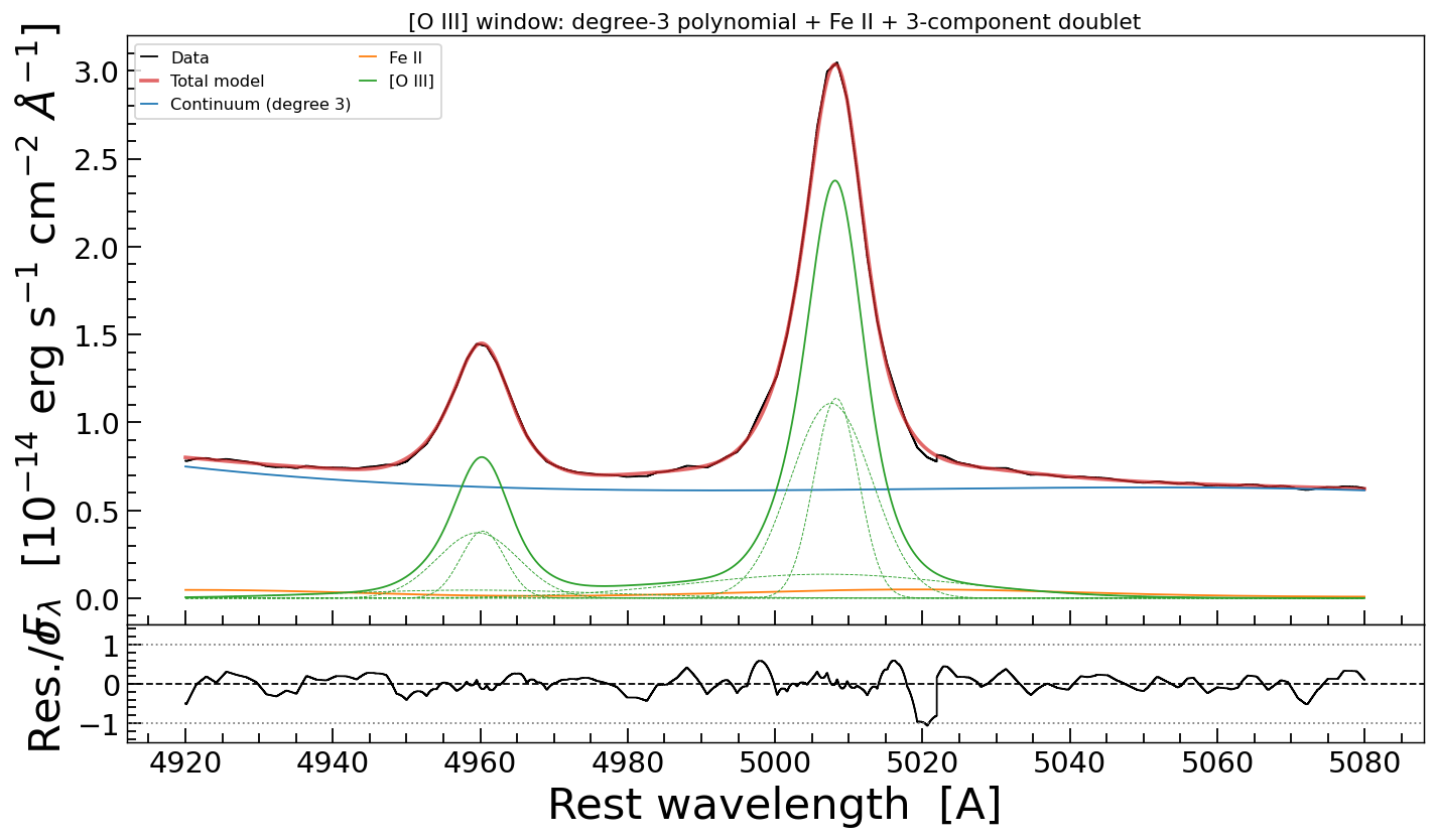
The [O III] window fit: data, total model, the degree-3 continuum, the iron, and the
three dashed curves that are the doublet’s core and two winds. Residuals in units of
the error in the lower panel. Drawn by plot_fit_jax, which takes the dashed
curves from the submodels themselves.#
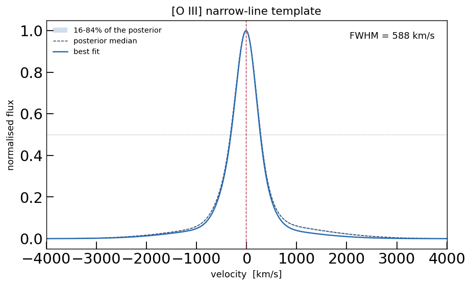
The profile that comes out: the fitted [O III] shape in velocity space, normalised to unit peak, with the half-maximum marked. FWHM 588 km/s, peak 9 km/s blueward of the systemic velocity. The shaded 16-84% envelope of the posterior is +-1% of the peak – thinner than the line, and thinner than the plot’s own line width.#
That last sentence is the honest part of this step. The decomposition into a core and
two wings is degenerate: the three components trade amplitude against width at almost
constant likelihood, so the parameters of the decomposition are not individually
determined – the posterior envelope of the profile is +-1% of the peak. What is
determined is the shape they all share, and that is the only thing the template uses.
profile_envelope in the script measures that envelope by resampling the posterior
and printing it next to the profile, so “the shape is safe to freeze” is a number and
not an assumption.
The script then writes the profile to example/data/iras07546_narrow_template.txt
with its provenance on top, so that a reader who finds only the file still knows where
it came from:
# narrow-line template of IRAS 07546+3928
# measured on the [O III] 4959/5007 doublet, normalised to unit peak
# generated by example/fit_iras07546_o3_template.py
# window 4920-5080 A, degree-3 local continuum, 3-component doublet, ln Z = 7450.85
# FWHM 587.9 km/s  (sigma_equivalent 249.6 km/s), peak at -9.0 km/s
# the frozen profile fits the window at chi2/dof = 0.086
# col 1: velocity [km/s]   col 2: normalised flux
The chi2/dof line is a self-consistency check, not a victory: the same window is
refitted with the frozen profile in place of the three Gaussians, and if the profile
were a poor description of the data this number would be orders of magnitude above the
0.086 the free fit reaches. The frozen profile is a smoother description, so it is not
expected to be identical – only close.
3. Build the model, one component at a time#
The whole-spectrum model is seventeen additive components of three kinds: a power-law
continuum, the Fe II template, and fifteen lines. An astropy model composes with +,
a galspec.jax_models model composes the same way, so the model is built by naming the
parts one after another and summing them. There is no builder function, and every piece
stays a model object that can be called on a wavelength array on its own – which is what
lets the four figures below draw each chunk of the model from the fitted parameters.
3.1. The continuum#
One power law over 2 600 A: an amplitude and a slope. It is anchored at 5500 A, in the middle of the range, so that amplitude and slope are nearly independent – move the anchor to the blue end and the two parameters become a line’s intercept and gradient, correlated at the 0.99 level.
# %% model_continuum
# ---- the continuum: one power law over 2600 A, anchored at 5500 A -------------------
continuum = jxm.PowerLaw1D(amplitude=0.55, x_0=5500.0, alpha=1.0,
                           fixed={"x_0": True}, name="Continuum")
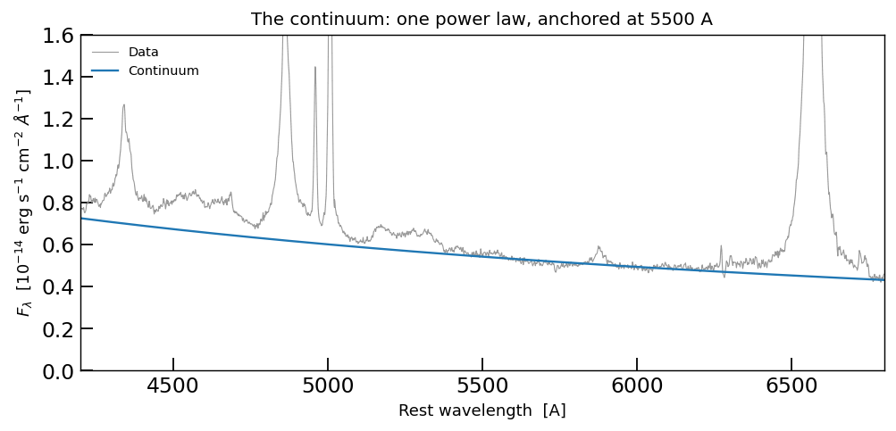
The continuum alone, drawn from the fitted parameters, against the data. alpha
comes out at 1.07 in F-lambda, which is a slope of -0.93 in F-nu – redder than a
bare quasar’s -0.5, the starburst showing through.#
3.2. The Fe II template#
The Fe II pseudo-continuum is not a line: it is a forest of blends between 4 200 and
5 600 A that no individual transition can be fitted. It is used as a template –
IronTemplate_tied – convolved with a broadening kernel and scaled by one number.
It is not a small correction: in the fit below it reaches 0.18 at 4 556 A against a
continuum of 0.66, a quarter of the total, and that structure has to go somewhere. A
model without it gives the flux to whatever else is nearby – the continuum, or a wing
on the nearest broad line.
The kernel is a Line_MultiGauss the compound model does not own; its parameters are
tied in section 4.3, which is why the iron costs exactly one free parameter – its
amplitude.
# %% model_iron
# ---- the iron pseudo-continuum ------------------------------------------------------
# IronTemplate_tied convolves the optical Fe II template with a Line_MultiGauss kernel it
# does not own: the kernel's parameters are tied to broad H-alpha below, so the iron costs
# exactly one free parameter -- its amplitude.
iron = jxm.IronTemplate_tied(n_components=2, amplitude=0.2, z=0.0,
                             dv_c=0.0, sigma_c=1500.0,
                             amp_w0=0.10, dv_w0=0.0, sigma_w0=6000.0, name="FeII")
iron.z.fixed = True                 # the redshift is the rest frame we are fitting in
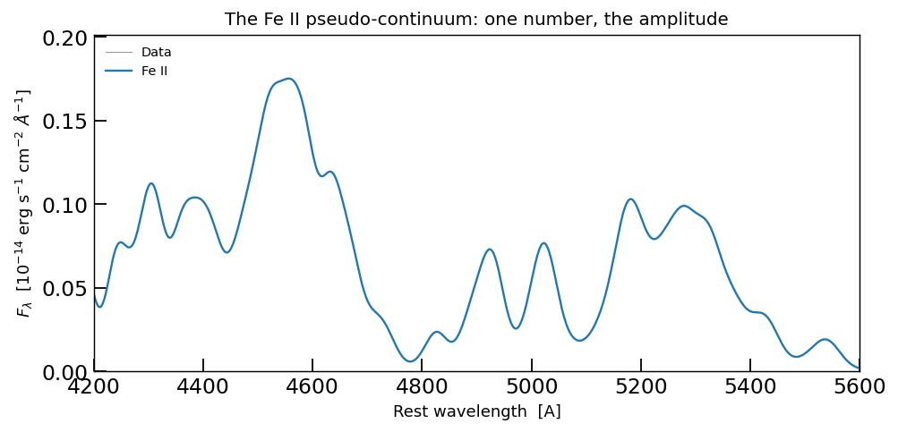
The Fe II pseudo-continuum under H-beta, [O III] and H-gamma, from the fitted amplitude. The wiggles are the template’s own structure; what the fit decides is the broadening (section 4.3) and the amplitude.#
3.3. The broad lines#
Three Balmer lines and two helium lines. Each Balmer line is a core plus a wind:
n_components=2 puts amp_c/dv_c/sigma_c and
amp_w0/dv_w0/sigma_w0 in one constructor call. He I 5876 and He II 4686 are
weak enough to be one Gaussian each.
What is not in this cell is as important as what is: no ties yet. The pieces are built loose and tied afterwards, because a tie resolves its reference by name at evaluation time and does not need the compound model to exist.
# %% model_broad
# ---- the broad lines: a core plus one wind each -------------------------------------
# ``n_components=2`` means a core and one wind: amp_c/dv_c/sigma_c and amp_w0/dv_w0/sigma_w0.
# The wind amplitudes are free per line (that is the Balmer decrement); shifts and widths
# are tied to broad H-alpha a few cells below.
b_halpha = jxm.Line_MultiGauss(n_components=2, wavec=LINE_WAVE["Halpha"], name="b_halpha",
                               amp_c=0.65, dv_c=0.0, sigma_c=1500.0,
                               amp_w0=0.10, dv_w0=0.0, sigma_w0=6000.0)
b_hbeta = jxm.Line_MultiGauss(n_components=2, wavec=LINE_WAVE["Hbeta"], name="b_hbeta",
                              amp_c=0.22, dv_c=0.0, sigma_c=1500.0,
                              amp_w0=0.20, dv_w0=0.0, sigma_w0=6000.0)
b_hgamma = jxm.Line_MultiGauss(n_components=2, wavec=LINE_WAVE["Hgamma"], name="b_hgamma",
                               amp_c=0.10, dv_c=0.0, sigma_c=1500.0,
                               amp_w0=0.20, dv_w0=0.0, sigma_w0=6000.0)
# He I 5876 and He II 4686 are weak enough to be one Gaussian each
b_hei = jxm.Line_MultiGauss(n_components=1, wavec=LINE_WAVE["HeI_5876"], name="b_hei",
                            amp_c=0.06, dv_c=0.0, sigma_c=1500.0)
b_heii = jxm.Line_MultiGauss(n_components=1, wavec=LINE_WAVE["HeII_4686"], name="b_heii",
                             amp_c=0.05, dv_c=0.0, sigma_c=1500.0)
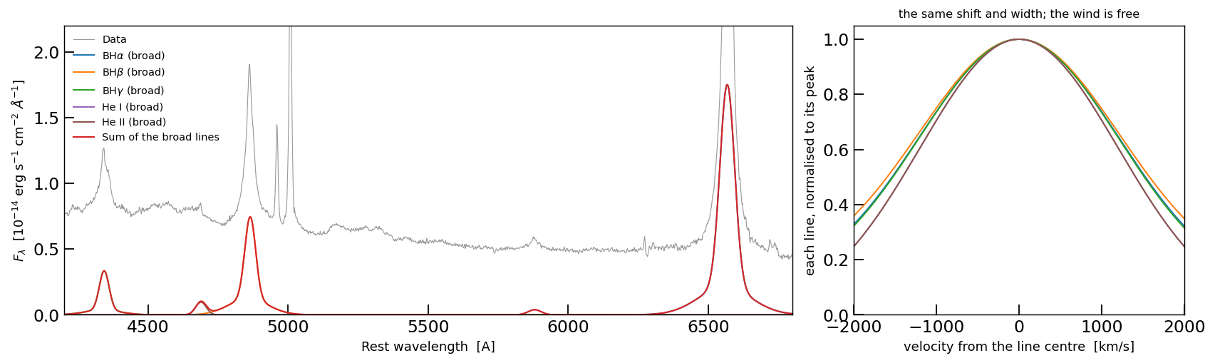
Left: the five broad components and their sum, from the fitted parameters. Right: the same five lines aligned on their peaks and normalised. The shift and the width are shared, so the curves nearly coincide; what separates them is the wind amplitude, which is free per line – the Balmer decrement of the wind, and a measurement.#
3.4. The narrow lines#
Ten lines, all on the measured profile. The template is read from the file and handed to
each line as template_velc and template_flux; a line that uses it has an amplitude
and a shift, and no width anywhere, because the profile carries it. A forbidden doublet is
one component with two peaks: the second amplitude is the atomic ratio (tied in section 4)
or, for [S II], free, because 6716/6731 measures the electron density.
# %% model_narrow
# ---- the narrow lines, all on one measured profile ----------------------------------
# The template is a single-line profile in velocity space, extracted from the [O III]
# doublet by example/fit_iras07546_o3_template.py and normalised to unit peak. A line that
# uses it has an amplitude and a shift -- no width is fitted anywhere.
profile = np.loadtxt(TEMPLATE_FILE, comments="#")
velc, tflux = profile[:, 0], profile[:, 1]
assert profile.shape[1] == 2
assert np.all(np.diff(velc) > 0) and np.allclose(np.diff(velc), np.diff(velc)[0],
                                                rtol=1e-6)   # a uniform grid

n_halpha = jxm.Line_template(template_velc=velc, template_flux=tflux,
                             wavec=LINE_WAVE["Halpha"], name="n_halpha",
                             amplitude=2.2, dv=0.0)
n_hbeta = jxm.Line_template(template_velc=velc, template_flux=tflux,
                            wavec=LINE_WAVE["Hbeta"], name="n_hbeta",
                            amplitude=0.8, dv=0.0)
n_hgamma = jxm.Line_template(template_velc=velc, template_flux=tflux,
                             wavec=LINE_WAVE["Hgamma"], name="n_hgamma",
                             amplitude=0.4, dv=0.0)
n_hei = jxm.Line_template(template_velc=velc, template_flux=tflux,
                          wavec=LINE_WAVE["HeI_5876"], name="n_hei",
                          amplitude=0.12, dv=0.0)
HeII = jxm.Line_template(template_velc=velc, template_flux=tflux,
                         wavec=LINE_WAVE["HeII_4686"], name="HeII",
                         amplitude=0.08, dv=0.0)
OIII4363 = jxm.Line_template(template_velc=velc, template_flux=tflux,
                             wavec=LINE_WAVE["OIII_4363"], name="OIII4363",
                             amplitude=0.05, dv=0.0)

# A forbidden doublet is one component with two peaks: the second amplitude is either the
# atomic ratio (tied below) or, for [S II], free -- 6716/6731 is a density diagnostic.
OIII = jxm.Line_template_doublet(template_velc=velc, template_flux=tflux,
                                 wavec0=LINE_WAVE["OIII_5007"],
                                 wavec1=LINE_WAVE["OIII_4959"], name="OIII",
                                 amp_c0=1.8, amp_c1=1.8 / 2.98, dv_c=0.0)
NII = jxm.Line_template_doublet(template_velc=velc, template_flux=tflux,
                                wavec0=LINE_WAVE["NII_6583"],
                                wavec1=LINE_WAVE["NII_6548"], name="NII",
                                amp_c0=1.0, amp_c1=1.0 / 2.96, dv_c=0.0)
SII = jxm.Line_template_doublet(template_velc=velc, template_flux=tflux,
                                wavec0=LINE_WAVE["SII_6716"],
                                wavec1=LINE_WAVE["SII_6731"], name="SII",
                                amp_c0=0.10, amp_c1=0.10, dv_c=0.0)
OI = jxm.Line_template_doublet(template_velc=velc, template_flux=tflux,
                               wavec0=LINE_WAVE["OI_6300"],
                               wavec1=LINE_WAVE["OI_6364"], name="OI",
                               amp_c0=0.05, amp_c1=0.05 / 3.0, dv_c=0.0)
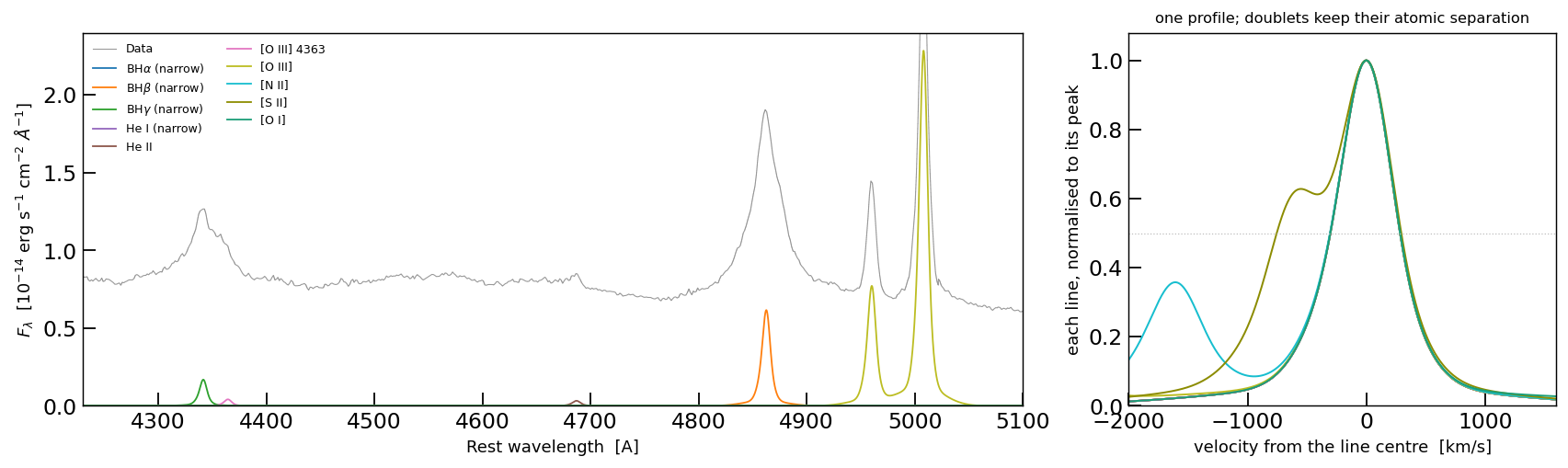
Left: where the ten narrow lines sit, each with its amplitude from the fit. Right: the same ten, aligned on their peaks and normalised – one curve, not ten, which is the whole point of the template. The offset curves are the doublets keeping their atomic separation: [N II] at -1 594 km/s, [S II] at -670 km/s.#
3.5. The sum#
The seventeen pieces are summed in a fixed order – narrow and broad alternating, so that a
reader finds [O III] next to H-beta rather than in a block at the end – and then given
display names, because a legend should say BH$\alpha$ (broad) and not b_halpha.
# %% model_sum
# ---- seventeen components, summed in the order a reader looks for them --------------
model = (continuum + iron
         + n_halpha + b_halpha + n_hbeta + b_hbeta + n_hgamma + b_hgamma
         + OIII + NII + SII + OI
         + HeII + b_heii + OIII4363 + n_hei + b_hei)

# display names, so a legend says "BH$\alpha$ (broad)" and not "b_halpha"
MODEL_LABELS = {
    "Continuum": "Continuum", "FeII": "Fe II",
    "n_halpha": r"BH$\alpha$ (narrow)", "b_halpha": r"BH$\alpha$ (broad)",
    "n_hbeta": r"BH$\beta$ (narrow)", "b_hbeta": r"BH$\beta$ (broad)",
    "n_hgamma": r"BH$\gamma$ (narrow)", "b_hgamma": r"BH$\gamma$ (broad)",
    "n_hei": "He I (narrow)", "b_hei": "He I (broad)", "b_heii": "He II (broad)",
    "OIII": "[O III]", "NII": "[N II]", "SII": "[S II]", "OI": "[O I]",
    "OIII4363": "[O III] 4363", "HeII": "He II",
}
for name, label in MODEL_LABELS.items():
    model[name].label = label

print(f"{len(model.submodel_names)} components, "
      f"{len(model.free_param_names)} free parameters before tying")
4. The ties#
A tie is not a constraint in the sampler: it removes a parameter. The tied parameter is
computed from another model’s parameter at evaluation time, so the sampler never sees it
and no likelihood penalty enforces it. The jxm.tie.* objects look the reference up by
name, which is why they can be assigned before or after the pieces are summed.
4.1. Tying the narrow lines: one shift, one ratio per doublet#
The narrow lines share a velocity: eleven peaks become one measurement of the narrow-line-region systemic velocity, and no line can drift on its own. The second peak of a forbidden doublet is not fitted at all, because the ratio is atomic.
# %% ties_narrow
# ---- one velocity for all ten narrow lines ------------------------------------------
for line in (n_halpha, n_hbeta, n_hgamma, n_hei, HeII, OIII4363):
    line.dv.tied = jxm.tie.tie_MultiGauss_dv_c("OIII")       # singlet: `dv`
for line in (NII, SII, OI):
    line.dv_c.tied = jxm.tie.tie_MultiGauss_dv_c("OIII")     # doublet: `dv_c`

# the second peak of a forbidden doublet is atomic physics, so it is tied, not fitted
OIII.amp_c1.tied = jxm.tie.tie_MultiGauss_doublet_ratio("OIII", 2.98)
NII.amp_c1.tied = jxm.tie.tie_MultiGauss_doublet_ratio("NII", 2.96)
OI.amp_c1.tied = jxm.tie.tie_MultiGauss_doublet_ratio("OI", 3.00)
# [S II] keeps both amplitudes free: 6716/6731 measures the electron density
Tying every narrow shift is a statement rather than a measurement: a line that really sits at a different velocity is absorbed into its amplitude and into the residual, and the model cannot report it. These lines do come from the same gas, so it is a good bet – but it is the kind of assumption worth writing down rather than leaving implicit in the code. The right-hand panel of the narrow-line figure above is what it buys: ten curves that are one curve.
4.2. Tying the broad lines: one shape, three amplitudes#
Broad H-beta and H-gamma follow H-alpha component by component: the core’s shift and width, and every wind’s shift and width. What is not tied is the amplitude, of the core or of the wind – the Balmer decrement is a measurement, and it is one of the things this fit is for.
# %% ties_broad
# ---- H-beta and H-gamma follow H-alpha, component by component ----------------------
# Core shift and width, then the wind's shift and width. What is left free is the
# amplitude of each -- the Balmer decrement is a measurement, not an assumption.
for line in (b_hbeta, b_hgamma):
    line.dv_c.tied = jxm.tie.tie_MultiGauss_dv_c("b_halpha")
    line.sigma_c.tied = jxm.tie.tie_MultiGauss_sigma_c("b_halpha")
    line.dv_w0.tied = jxm.tie.tie_MultiGauss_dv_w0("b_halpha")
    line.sigma_w0.tied = jxm.tie.tie_MultiGauss_sigma_w0("b_halpha")
for line in (b_hei, b_heii):
    line.dv_c.tied = jxm.tie.tie_MultiGauss_dv_c("b_halpha")
    line.sigma_c.tied = jxm.tie.tie_MultiGauss_sigma_c("b_halpha")

print(f"{len(model.free_param_names)} free parameters after tying")
This is the “one broad-line region” assumption, and it is the one
example/fit_iras07546_jax_tied.py tests: that script releases the eight parameters
removed here, puts a Gaussian on the difference instead of a tie, and reports how far
each line moved in units of that width (Priors has the construction and the
result – H-gamma’s wind is the one that disagrees).
4.3. Tying the iron template: its kernel is broad H-alpha#
The iron is a template convolved with a broadening kernel. Every parameter of that kernel – core shift and width, wind shift and width – is tied to the broad H-alpha component, which is the strongest statement in the model: the iron lines come from the same gas as the Balmer line, so they cannot have a velocity structure the Balmer line does not have.
# %% ties_iron
# ---- the iron kernel is broad H-alpha, parameter for parameter ----------------------
iron.dv_c.tied = jxm.tie.tie_MultiGauss_dv_c("b_halpha")
iron.sigma_c.tied = jxm.tie.tie_MultiGauss_sigma_c("b_halpha")
iron.amp_w0.tied = jxm.tie.tie_MultiGauss_amp_w0("b_halpha")
iron.dv_w0.tied = jxm.tie.tie_MultiGauss_dv_w0("b_halpha")
iron.sigma_w0.tied = jxm.tie.tie_MultiGauss_sigma_w0("b_halpha")

print(f"{len(model.free_param_names)} free parameters in the model that is fitted")
Why tie rather than fit the kernel? Because a free kernel width lets the iron absorb Fe II flux into a fake wind, and earlier fits of this object did exactly that – the narrow lines were fitted well and the broad profile was quietly wrong. With the kernel tied, the iron costs exactly one free parameter, its amplitude.
The three cells of this section take the model from 56 parameters to 32 (the narrow ties) to 27 (the broad and iron ties); the printouts at the end of each one say so.
5. A prior for every parameter#
One prior per free parameter, and every one of them is scaled from the spectrum rather than copied from a previous fit, so the recipe transfers to another object without hand-tuning.
Two shapes do the work. LogUniform gives equal probability per factor of ten, which is
what a line peak that may be four decades fainter than the brightest pixel needs – a
linear box would put 99% of its prior at the bright end and never visit the faint lines.
Uniform is right for a quantity whose natural range is already the physical one: a
velocity shift, a width, or a ratio bounded by 1.
The dictionary is written out parameter by parameter, because that is the thing a reader edits to fit their own object; the loop after it is the entire mechanism. It ends by walking every free parameter and asserting that each one has a prior: a fit with an unset prior is a silent bug – the parameter samples its whole default box – and the assertion turns that into an error before the sampler starts.
# %% priors
# ---- one prior per free parameter, scaled from the spectrum -------------------------
peak = float(np.max(flux))                       # the brightest pixel
continuum = float(np.percentile(flux, 15.0))     # the line-free level
amp = (1e-3, 3.0 * peak)                         # a line peak: invisible to 3x the peak

PRIORS = {                        # [output] qualified name -> (shape, lower, upper)
    "Continuum.amplitude":  ("log", 0.2 * continuum, 4.0 * continuum),
    "Continuum.alpha":      ("uniform", -5.0, 5.0),
    "FeII.amplitude":       ("log", 1e-3, 3.0 * continuum),

    "n_halpha.amplitude":   ("log", *amp),
    "n_hbeta.amplitude":    ("log", *amp),
    "n_hgamma.amplitude":   ("log", *amp),
    "n_hei.amplitude":      ("log", *amp),
    "HeII.amplitude":       ("log", *amp),
    "OIII4363.amplitude":   ("log", *amp),
    "OIII.amp_c0":          ("log", *amp),
    "NII.amp_c0":           ("log", *amp),
    "SII.amp_c0":           ("log", *amp),
    "SII.amp_c1":           ("log", *amp),         # [S II]: both peaks free
    "OI.amp_c0":            ("log", *amp),

    "OIII.dv_c":            ("uniform", -1000.0, 1000.0),   # the narrow-line systemic

    "b_halpha.amp_c":       ("log", *amp),
    "b_halpha.dv_c":        ("uniform", -2500.0, 2500.0),
    "b_halpha.sigma_c":     ("uniform", 300.0, 8000.0),
    "b_halpha.amp_w0":      ("uniform", 0.0, 1.0),          # the wind: a ratio to the core
    "b_halpha.dv_w0":       ("uniform", -6000.0, 6000.0),
    "b_halpha.sigma_w0":    ("uniform", 300.0, 8000.0),
    "b_hbeta.amp_c":        ("log", *amp),
    "b_hbeta.amp_w0":       ("uniform", 0.0, 1.0),
    "b_hgamma.amp_c":       ("log", *amp),
    "b_hgamma.amp_w0":      ("uniform", 0.0, 1.0),
    "b_hei.amp_c":          ("log", *amp),
    "b_heii.amp_c":         ("log", *amp),
}

for name, (shape, low, high) in PRIORS.items():
    submodel, parameter = name.split(".", 1)
    getattr(model[submodel], parameter).prior = (priors.LogUniform(low, high) if shape == "log"
                                                 else priors.Uniform(low, high))

# check it: no free parameter may be left without a prior
free = set(model.free_param_names)
pairs = list(zip(model.param_names, model.qualified_param_names))
unset = [q for flat, q in pairs if flat in free and q not in PRIORS]
print(f"{len(PRIORS)} priors for {len(free)} free parameters; unset: {unset}")
assert not unset
The recipe is written out on Priors, which also explains what each shape does and how to make one parameter’s prior depend on another’s.
6. Run the sampler#
Nested sampling on the GPU. nlive live points are drawn from the prior and the worst
one is repeatedly replaced with a point of higher likelihood: the volume shrinks, the
likelihood rises, and the integral of both is the evidence. The surviving points are a
weighted sample of the posterior, which is what everything below quotes. The run stops
when less than dlogz of the evidence may remain unseen.
# %% sampler
nlive, dlogz = (120, 0.5) if QUICK else (NLIVE, DLOGZ)
fit = JNesty_Fit(model, wave, flux, error, nlive=nlive, bound="multi", device=DEVICE)
print(f"fit: {nlive} live points, dlogz {dlogz}, device {fit.device}  [{jax_devices_summary()}]")
Before spending the runtime, a check: draw parameter sets from the priors alone and look at the band they span. If the data sit inside it, the prior contains the answer – which is why no least-squares seed is needed and the starting values in the model do not matter.
# %% prior_check
model.prepare(wave)
rng = np.random.default_rng(0)
theta_prior = np.array([fit.prior_transform(row) for row in rng.random((120, fit.ndim))])
draws = np.asarray(model.flux_batch(wave, theta_prior))

step = slice(None, None, 11)
fig, ax = plt.subplots(figsize=(13.0, 3.8), constrained_layout=True)
ax.fill_between(wave[step], np.percentile(draws, 1, axis=0)[step],
                np.percentile(draws, 99, axis=0)[step], color="#2b6cb0", alpha=0.18,
                label="1-99% of 120 draws from the priors")
ax.plot(wave[step], flux[step], color="0.35", lw=0.6, label="data")
for centre in (LINE_WAVE["Hgamma"], LINE_WAVE["Hbeta"],
               LINE_WAVE["HeI_5876"], LINE_WAVE["Halpha"]):
    ax.axvline(centre, color="#b5364a", lw=0.6, ls=":")
ax.set_yscale("symlog", linthresh=1.0)
ax.set_xlabel("rest wavelength  [A]")
ax.set_ylabel(FLUX_LABEL)
ax.set_title("The priors alone already bracket the spectrum")
ax.legend(fontsize=9, frameon=False);
# %% run
started = time.perf_counter()
fit.fit(progress=sys.stdout.isatty(), dlogz=dlogz, max_iterations=MAX_ITERATIONS)
print(f"\n  log Z = {fit.log_evidence:.2f} +- {fit.log_evidence_err:.2f}"
      f"   ({fit.n_iterations} iterations, {(time.perf_counter() - started) / 60:.1f} min)")
It prints:
log Z = 130678.63 +- 0.58 (59786 iterations, 7.9 min)
and the next cell adds the residual:
chi2/dof = 0.315, residual rms 0.56 sigma, worst pixel 3.9 sigma
JNesty seeds its live points from a fixed key, so a rerun visits the same points. That is not bitwise identity – the same fit run twice comes out a nat apart, from the last bits of a float sum feeding the sampler’s ordering – but it does mean the quoted uncertainty is the sampler’s error bar, and the run-to-run scatter sits well inside it.
7. Present the results#
The table is the answer: posterior median and the 16th/84th percentiles, a 68% credible interval, the Bayesian counterpart of “1 sigma”.
# %% table
# ---- the fit, and the parameter table ----------------------------------------------
model_best, _, theta = fit.get_best_fit()
predicted = np.asarray(model_best.flux(wave, theta))
residual = (flux - predicted) / error
dof = wave.size - len(theta)
chi2_dof = float(np.sum(residual ** 2) / dof)
print(f"  chi2/dof = {chi2_dof:.3f}, residual rms {residual.std():.2f} sigma, "
      f"worst pixel {np.abs(residual).max():.1f} sigma")

# a unit per parameter, read off the suffix of its name
UNITS = {"amp_w": "ratio to core", "amp_c": "1e-14 erg/s/cm2/A",
         "amplitude": "1e-14 erg/s/cm2/A", "dv": "km/s", "sigma": "km/s"}
lo, med, hi = fit.get_quantiles((0.16, 0.5, 0.84))
print(f"\n  {'parameter':22s} {'median':>10s} {'-':>9s} {'+':>9s}  unit")
print("  " + "-" * 74)
for index, name in enumerate(fit.full_param_names):
    base = name.split(".", 1)[-1]
    unit = next((text for stem, text in UNITS.items() if base.startswith(stem)), "-")
    print(f"  {name:22s} {med[index]:10.5g} {med[index] - lo[index]:9.2g} "
          f"{hi[index] - med[index]:9.2g}  {unit}")
Read it with the ties in mind – OIII.dv_c is the shift of every narrow line, and
b_halpha.sigma_w0 is the width of the wind in all three Balmer lines, in He I and in
the Fe II kernel. The unit column is read off the parameter’s suffix, so nothing has to be
remembered: amp* is a flux density, dv*/sigma* is km/s, amp_w* is a ratio to
the core.
Note what is not in the table: any narrow-line width. The ten narrow lines contribute twelve numbers – eleven peaks (six singlets, four doublet main peaks and both peaks of [S II]) and one shared shift – where a Gaussian per line spends a width on top of that. The 27-parameter count against the published model’s 30 comes from exactly there.
The comparison against the published model, and the widths and fluxes a paper would quote:
# %% scoreboard
# ---- and the number that says whether the measured profile was worth it -------------
# The published fit is the same spectrum, continuum, broad lines and priors, with a Gaussian
# per narrow line and one width shared between them. Nested sampling compares models by their
# evidence, so this is the comparison that matters.
REFERENCE = {
    "published": {"free_parameters": 30, "log_evidence": 130889.60, "chi2_dof": 0.307},
    "template":  {"free_parameters": 27, "log_evidence": 130677.27, "chi2_dof": 0.315},
}
this_run = dict(REFERENCE["template"], free_parameters=len(theta),
                log_evidence=fit.log_evidence, chi2_dof=chi2_dof)

print(f"\n  {'model':26s} {'free':>5s} {'ln Z':>12s} {'chi2/dof':>9s}")
print("  " + "-" * 56)
for label, row in list(REFERENCE.items()) + [("this run", this_run)]:
    mark = "*" if label == "this run" else " "
    print(f" {mark}{label:26s} {row['free_parameters']:5d} "
          f"{row['log_evidence']:12.2f} {row['chi2_dof']:9.3f}")
delta = this_run["log_evidence"] - REFERENCE["published"]["log_evidence"]
print(f"  {'':27s} {'':5s} Delta = {delta:+.2f} nats against the published Gaussian model")
# %% fluxes
# ---- widths and integrated fluxes, per posterior sample ----------------------------
# A flux is a combination of parameters, so it is computed for every sample rather than from
# the medians: that is how its error bar inherits the correlations in the fit.
FWHM = 2.0 * np.sqrt(2.0 * np.log(2.0))       # sigma -> FWHM
C_KM_S = 299792.458

samples = np.asarray(fit.samples_equal_weight, dtype=float)
column = {name: index for index, name in enumerate(fit.full_param_names)}


# A Gaussian's integral is ``A sigma sqrt(2 pi)`` when the width is in wavelength, so the
# velocity width is converted first: one km/s is ``wavelength / c`` Angstrom.
core = (samples[:, column["b_halpha.amp_c"]]
        * samples[:, column["b_halpha.sigma_c"]] * LINE_WAVE["Halpha"] / C_KM_S
        * np.sqrt(2.0 * np.pi) * 1e3)
# the wind is a ratio to the core, so its flux is the core's times the ratio of its width
# to the core's -- the amplitudes already differ by that ratio
wind = (samples[:, column["b_halpha.amp_w0"]]
        * samples[:, column["b_halpha.sigma_w0"]] / samples[:, column["b_halpha.sigma_c"]]
        * core)

# the template's area on the velocity grid: the same for every narrow line, read once
narrow_velc = np.asarray(model["OIII"]._template_velc)
narrow_shape = np.asarray(model["OIII"]._template_flux)
narrow_area = np.trapezoid(narrow_shape, narrow_velc)            # km/s per unit peak
narrow_flux = samples[:, column["n_halpha.amplitude"]] * narrow_area \
    * LINE_WAVE["Halpha"] / C_KM_S * 1e3

peak_i = int(np.argmax(narrow_shape))
left = np.interp(0.5, narrow_shape[peak_i::-1], narrow_velc[peak_i::-1])
right = np.interp(0.5, narrow_shape[peak_i:][::-1], narrow_velc[peak_i:][::-1])

ROWS = [("broad H-alpha core", "b_halpha.sigma_c", core),
        ("broad H-alpha wind", "b_halpha.sigma_w0", wind),
        ("narrow H-alpha", None, narrow_flux)]
print(f"  {'component':22s} {'FWHM [km/s]':>12s}   {'flux [1e-17 erg/s/cm2]':>24s}")
print("  " + "-" * 62)
for label, width_name, flux_samples in ROWS:
    flux_lo, flux_med, flux_hi = np.percentile(flux_samples, [16, 50, 84])
    if width_name is None:
        width_text = f"{right - left:12.0f}"
    else:
        width = samples[:, column[width_name]] * FWHM
        width_lo, width_med, width_hi = np.percentile(width, [16, 50, 84])
        width_text = f"{width_med:8.0f} +{width_hi - width_med:.0f}/-{width_med - width_lo:.0f}"
    print(f"  {label:22s} {width_text:>12s}   "
          f"{flux_med:11.1f} +{flux_hi - flux_med:.1f}/-{flux_med - flux_lo:.1f}")
A flux is a combination of parameters, so it is computed per posterior sample rather than from the medians: that is how its error bar inherits the correlations in the fit. The narrow-line flux needs the template’s area on the velocity grid, which is read once off the profile – the same area for all ten lines, since they share the shape.
# %% fit_figure
fig = plt.figure(figsize=(17.0, 8.0))
ax = fig.add_axes([0.055, 0.20, 0.80, 0.72])
axr = fig.add_axes([0.055, 0.07, 0.80, 0.13])
galspec.plot.plot_fit_jax(wave, flux, model_best, ax=ax, axr=axr, error=error,
                          residual_in_sigma=True,
                          xlabel="Rest wavelength  [A]", ylabel=FLUX_LABEL,
                          legend_kwargs={"fontsize": 10, "ncol": 2,
                                         "loc": "center left",
                                         "bbox_to_anchor": (1.005, 0.5),
                                         "frameon": False})
ax.set_title("IRAS 07546+3928: narrow lines on the measured [O III] profile",
             fontsize=13)
fig.savefig(OUTPUT_DIR / "iras07546_jax_fit.png", dpi=150, bbox_inches="tight")
print(f"  wrote {OUTPUT_DIR / 'iras07546_jax_fit.png'}")
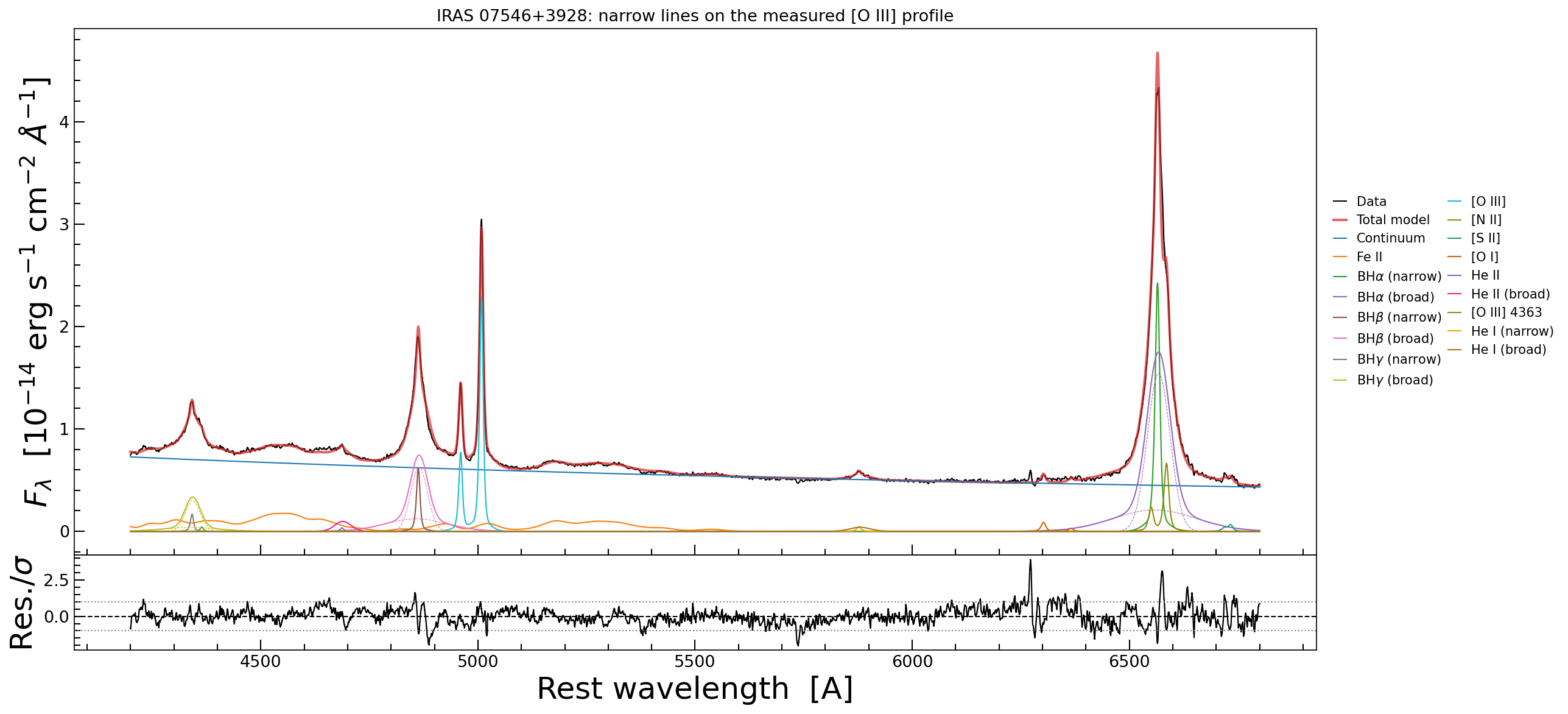
The full 4200-6800 A window: data, total model, and every component underneath it, with the broad lines’ cores and winds drawn as dashed curves in the colour of the line they belong to. The lower panel is the residual in units of the error, with the +-1 sigma guides.#
Three windows: 870 A, 380 A and 250 A wide, against the 2 600 A in the figure above. On that page a 700 km/s narrow core is two pixels; here it is a profile, and the wings of the broad lines are visible at all.
# %% zooms
# three windows, where the lines actually are
for tag, title, xlim, ylim in ZOOMS:
    ax, _ = galspec.plot.plot_fit_jax(wave, flux, model_best, error=error,
                                      xlim=xlim, ylim0=ylim, ylim1=(-8, 8),
                                      residual_in_sigma=True,
                                      xlabel="Rest wavelength  [A]", ylabel=FLUX_LABEL,
                                      legend_kwargs={"fontsize": 8, "ncol": 2,
                                                     "loc": "upper left",
                                                     "frameon": True})
    ax.figure.set_size_inches(13.5, 6)
    ax.set_title(f"{title}: {xlim[0]:.0f}-{xlim[1]:.0f} A", fontsize=13)
    ax.figure.savefig(OUTPUT_DIR / f"iras07546_jax_fit_{tag}.png", dpi=150,
                      bbox_inches="tight")
    print(f"  wrote {OUTPUT_DIR / f'iras07546_jax_fit_{tag}.png'}")
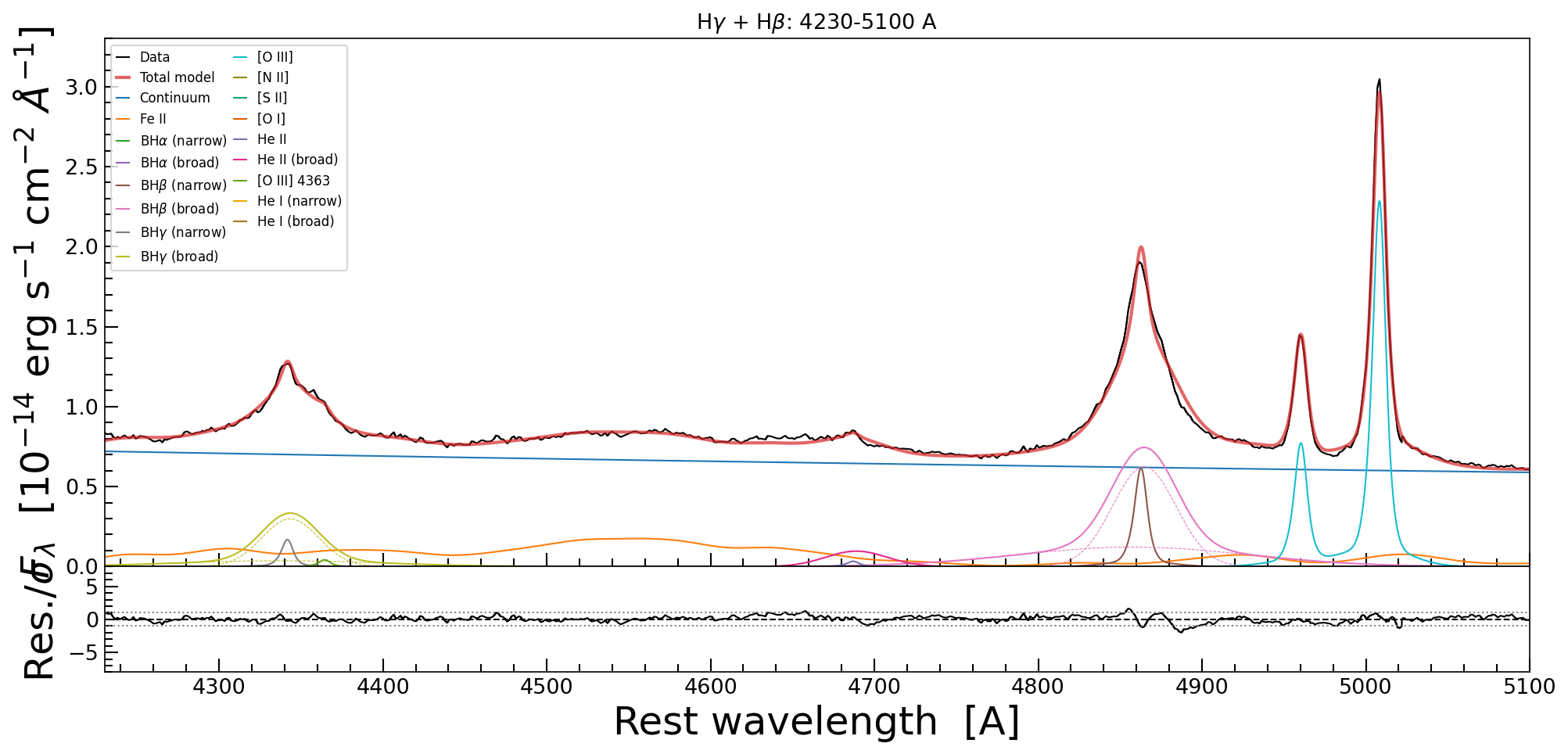
H-gamma + H-beta with the [O III] doublet.#
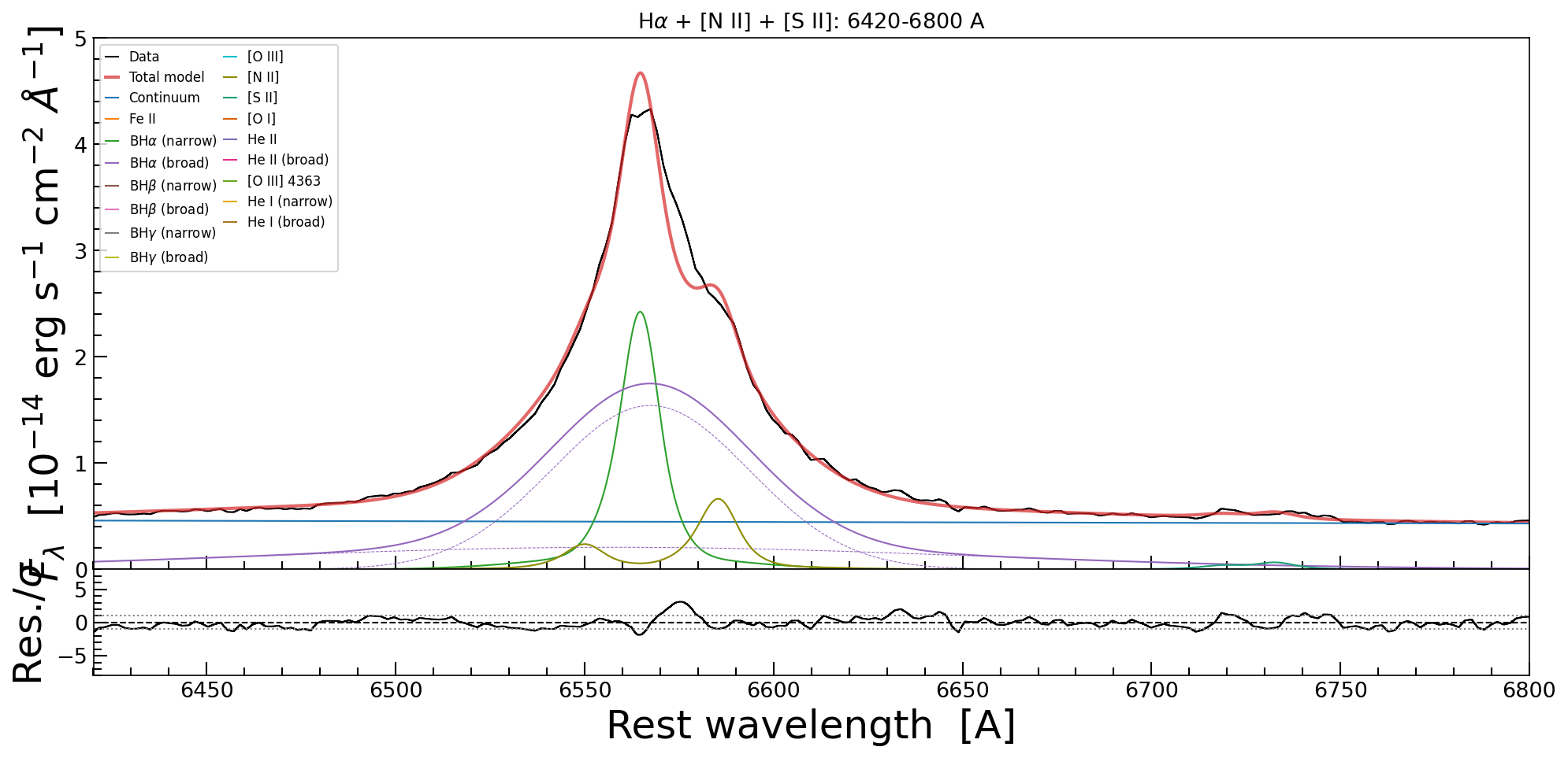
H-alpha with [N II] and [S II]. The narrow lines sit on broad wings that the model does not try to fit with the same component, and the two dashed purple curves are broad H-alpha’s core and wind, drawn separately.#
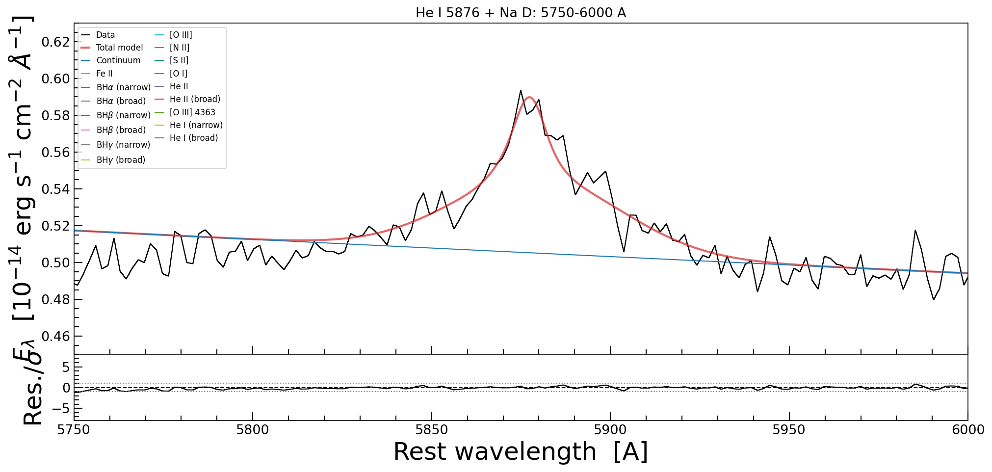
He I 5876 and Na D, the faintest features in the model.#
The posterior itself: one histogram per parameter, and the joint distribution of the parameters that a reader is most likely to want a covariance for.
# %% corner
# the joint posterior, for the fourteen parameters worth looking at together: a 27x27 square
# is unreadable
keep = [i for i, name in enumerate(fit.full_param_names) if name in CORNER_PARAMS]
labels = getattr(fit, "param_labels", None) or list(fit.full_param_names)
try:
    corner_fig = corner.corner(fit.samples_equal_weight[:, keep],
                               labels=[labels[i] for i in keep],
                               quantiles=(0.16, 0.5, 0.84), show_titles=True,
                               title_fmt=".3g", title_kwargs={"fontsize": 8})
except ValueError:
    print("  corner plot skipped: a selected parameter has no posterior range")
else:
    corner_fig.savefig(OUTPUT_DIR / "iras07546_jax_corner.png", dpi=110,
                       bbox_inches="tight")
    print(f"  wrote {OUTPUT_DIR / 'iras07546_jax_corner.png'}")
# %% histograms
# one histogram per number the fit exists for. The x range comes from the posterior, not from
# the prior: a width prior spans 300-8000 km/s while the posterior spans a few km/s, and an
# axis stretched to the prior would draw the measurement as a one-pixel spike.
galspec.plot.plot_posterior_hist(
    fit, params=HIST_PARAMS, ncols=4, bins=40,
    title="IRAS 07546+3928: marginal posteriors",
    filename=str(OUTPUT_DIR / "iras07546_jax_histograms.png"))
print(f"  wrote {OUTPUT_DIR / 'iras07546_jax_histograms.png'}")
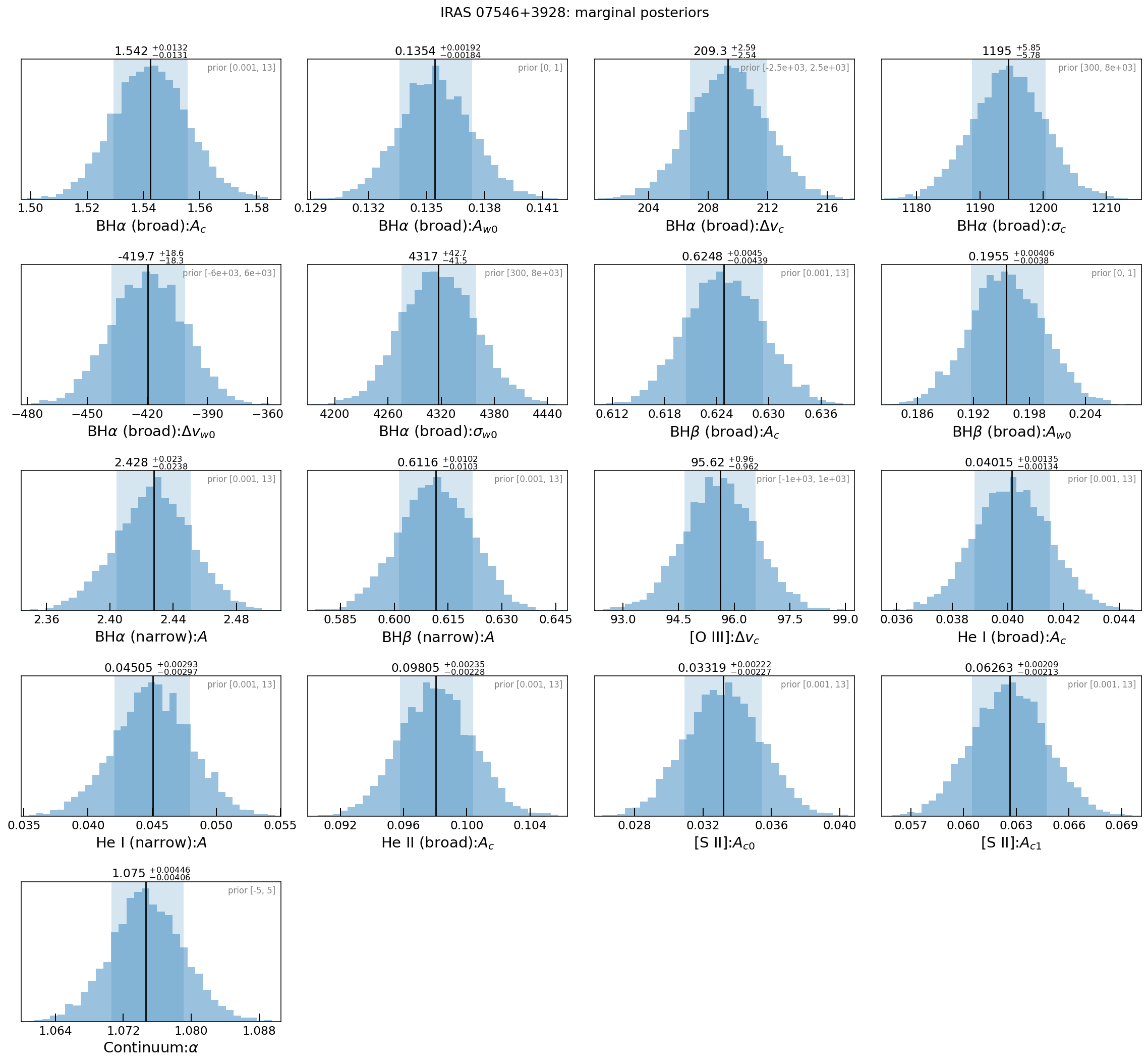
Marginal posteriors, with the prior range marked on each panel.#
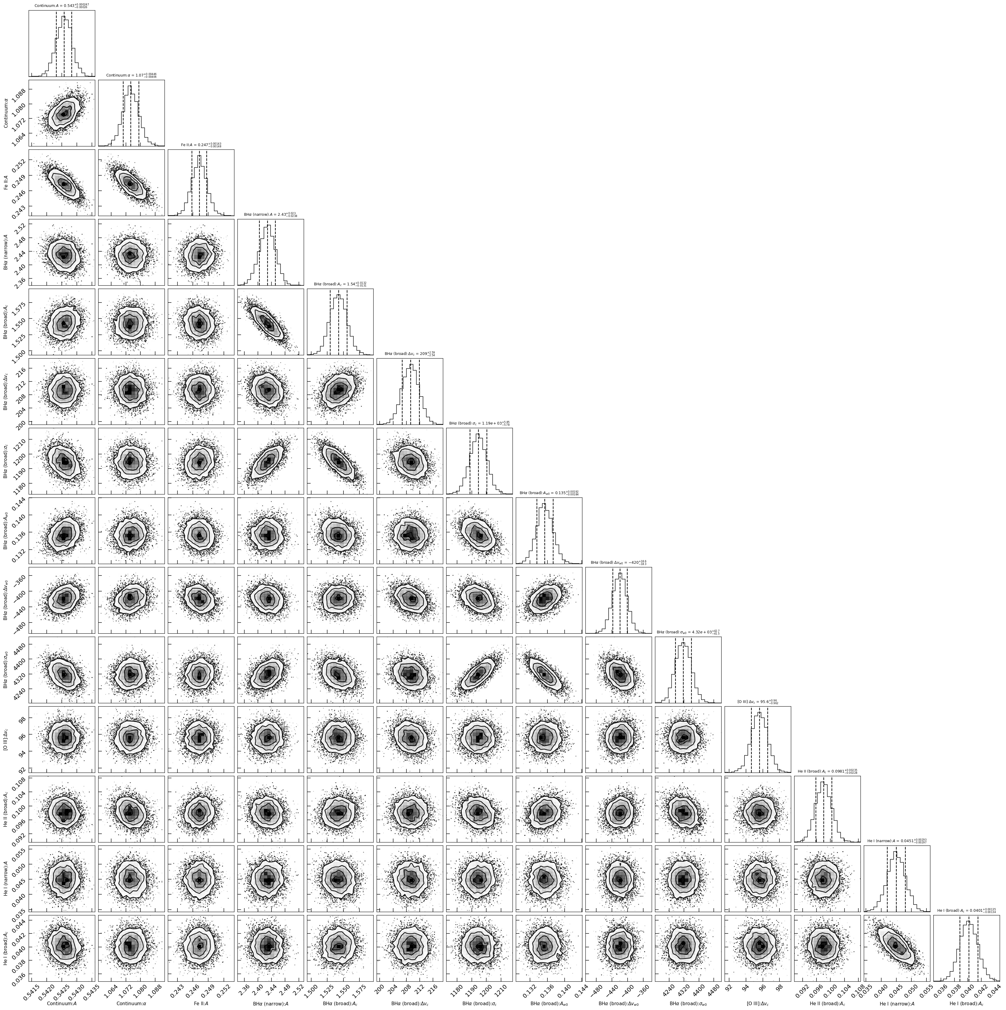
The joint posterior of the parameters the fit is most sensitive to.#
8. Save it, and read it back#
A nested-sampling run is expensive; the file should be the thing you keep. One FITS holds
the samples and their weights, their unit-cube coordinates, the evidence and its error, the
parameter names, bounds and priors, the sampler’s convergence trajectory, the model
description and the spectrum that was fitted – everything the figures above are drawn
from. Reloading gives a galspec.JNesty_Fit whose quantiles, best fit and plots work
unchanged.
# %% save
fits_path = OUTPUT_DIR / "iras07546_jax_fit.fits"
save_jnesty_fit_to_fits(fit, fits_path)
print(f"  wrote {fits_path}  ({fits_path.stat().st_size / 1e6:.0f} MB)")
print(f"  read it back with load_jnesty_fit_from_fits({str(fits_path)!r})")
fit.release_device_buffers()
# %% readback
loaded = load_jnesty_fit_from_fits(fits_path)

print(f"log Z stored    {fit.log_evidence:12.2f} +/- {fit.log_evidence_err:.2f}")
print(f"log Z reloaded  {loaded.log_evidence:12.2f} +/- {loaded.log_evidence_err:.2f}")
print("same parameters:", list(loaded.param_names) == list(fit.param_names))
print("same posterior: ", np.allclose(loaded.samples_equal_weight, fit.samples_equal_weight))

# the priors came back too, and the model knows which parameters are free
free = set(loaded.model.free_param_names)
pairs = list(zip(loaded.model.param_names, loaded.model.qualified_param_names))
print("priors restored:", all(loaded.model.get_prior(q) is not None
                              for flat, q in pairs if flat in free))
What is in the file – and the one thing that cannot be stored, a prior written as a plain Python function – is on JAX / GPU acceleration; the priors that went into it are on Priors. The same fit driven from a configuration file instead of a notebook is Fitting From a Configuration File: that is what to reach for when the model is the same and the spectra are many.
9. What the numbers say#
The comparison printed in section 7 is the point of writing the model this way:
 model                       free         ln Z  chi2/dof
 --------------------------------------------------------
 published                     30    130889.60     0.307
 template                      27    130677.27     0.315
*this run                      27    130678.63     0.315
                                    Delta = -210.97 nats against the published Gaussian model
The published model is the same spectrum, the same continuum, the same broad lines and
the same priors, with a Gaussian per narrow line and one width shared between them. The
only difference is the narrow-line profile, so the 211 nats are the price of that
assumption – not of the code: the templated model fits [O III] itself better, and a
second, independently written implementation of the same model agrees to a hundredth of
a nat. This run lands about a nat from the stored template row, inside its 0.58
error bar – see Priors on why the fixed key does not buy bitwise identity – and
re-extracting the template moves the evidence by more than that again, so the comparison
is between runs made on the same template file.
The reason is measurable rather than mysterious. The same local treatment applied to narrow H-alpha instead of [O III] gives a width of about 300 km/s, against an equivalent 249.6 km/s for the [O III] profile – a ratio of 0.84. The narrow Balmer lines in this object are broader than [O III], so a profile measured on [O III] and stamped under H-alpha, the strongest narrow line in the spectrum, under-fits it. The residual is not flat across that line: it runs at -0.6 sigma over the core and +2.3 sigma on the red shoulder (6570-6580 A), which is the signature of a shape very slightly too narrow and too peaked for this line – and it is what the H-alpha zoom above shows. A Gaussian model with one free common width can split the difference; a frozen profile cannot.
That ratio was measured with the portability check in
develop/dev_template/stage1_o3_template.py, the local script that also scanned the
component count; it is not part of this repository, so treat the number as provenance
rather than as something the page reproduces. That is a result about IRAS 07546+3928 and
a lesson about the method, and it is worth knowing before reaching for a template:
measure the profile on the line you trust, then check that the other lines share it.
For the forbidden lines alone, which do share their kinematics, the extraction is sound
and the model is the right one; for a Balmer-dominated narrow-line region, anchor the
template on a Balmer line instead.
The [S II] ratio that comes out of the fit is 0.0625/0.0333 = 1.88, measured rather than tied (it is a density diagnostic), and the [N II] and [O I] ratios are at their atomic values because nothing physical varies them.
Where to go next#
example/fit_iras07546_jax.ipynb: this page, cell by cell. Copy a cell, change a number, run it – the model has no builder function to look up.example/fit_iras07546_o3_template.py: step 2 on its own – the window fit, the profile, and the file the whole-spectrum fit reads.example/iras07546_model.py: the same model as an importable module, shared by the three fitting scripts.tests/test_example_notebook.pyholds it to the notebook.example/fit_iras07546_jax_tied.py: the same fit with the Balmer kinematics released and centred on H-alpha, which turns “the lines share one profile” into a measurement (Priors has the construction and the result).example/fit_iras07546_jax_toggle.py: how many broad components the profile needs, decided by the sampler rather than assumed – four on this object, with every sample agreeing (Priors has the numbers).Example: measure the black hole and the host galaxy: the other worked example – a low-luminosity AGN whose continuum is starlight rather than a power law, taken apart into host galaxy and nucleus and ending at a black-hole mass.
JAX / GPU acceleration: the JAX backend, the batching, and the CPU-versus-GPU comparison.