Example: measure the black hole and the host galaxy#

The other example fits a luminous AGN, where the continuum is a power law and the lines sit on top of it. This one goes the hard direction: a low-redshift SDSS spectrum in which the starlight is most of the light between 3900 and 7000 A, so the continuum has to be taken apart into five stellar populations and a nucleus before anything else can be measured. Two numbers come out of that decomposition – the stellar velocity dispersion and the 5100 A luminosity – and they, with the width of broad H-beta, give the black-hole mass.

Every code block on this page is a cell of example/fit_sdss0006_jax.ipynb, the notebook of the same name, so a block can be copied into a notebook and run:

example/fit_sdss0006_jax.ipynb – the whole analysis, cell by cell: four nested-sampling stages, the posterior of each, and the twelve figures below;
example/data/spec-0651-52141-0434.fits – the spectrum (SDSS plate 0651, MJD 52141, fibre 0434: 3 841 pixels from 3 806 to 9 215 A, with an inverse variance per pixel);
example/output/sdss0006_sii_template.txt – the narrow-line profile, written out at step 4 so that a reader who finds only the file knows where it came from.

SDSS J000605.59-092007.0, z = 0.0699. The object has broad H-alpha (FWHM ~ 2 900 km/s), narrow [O III]/H-beta ~ 5 and [N II]/H-alpha ~ 0.7 – a Seyfert 1 whose host is comparable to the nucleus at these wavelengths, which is what makes it the interesting case. The whole page runs in about ten minutes on one GPU.

The answer, first #

Four stages, each sampled separately, each with its own evidence:

stage 1   log Z = -2047.05 +- 0.12   the continuum: 5 stars + a power law, 9 free
stage 2   log Z =     -94.58 +- 0.08   [S II]: the narrow-line template, 7 free
stage 3   log Z =    -454.60 +- 0.11   the H-alpha complex, 8 free
stage 4   log Z =   -1070.14 +- 0.14   + H-beta and [O III], two windows, 14 free

and what they give:

sigma_*                   74.20 (-5.27/+5.56) km/s      <- stage 1
lambda L_lambda(5100)     2.27 (-0.28/+0.24) e42 erg/s  <- stage 1
FWHM(broad H-alpha)       2946 (-254/+300) km/s         <- stage 3
FWHM(broad H-beta)        3430 (-624/+716) km/s         <- stage 4
log [N II]/H-alpha        -0.133 (-0.152, -0.112)       <- stage 3
log [O III]/H-beta        +0.682 (+0.624, +0.745)       <- stage 4
log M_BH [M_sun]          7.10 (-0.17/+0.17)            <- stages 1 + 4

Read sigma_* with the caveat in section 5: it is the number in this list that a second run of the same stage does not reproduce, and the interval above is narrower than the run-to-run spread.

1. The spectrum #

Everything the notebook needs is set in one cell: the file, the redshift, the foreground extinction, the sampler’s two numbers and the device. The two sampler numbers are 2 000 live points and a 2% evidence tolerance, which is what every run quoted on this page used; QUICK = True drops them to 300 and 10% and fits the whole page in a minute, for checking that something runs rather than for a number.

# %% settings
# ---- what to fit, and where the answer goes -----------------------------------------
DATA_FILE = HERE / "data" / "spec-0651-52141-0434.fits"
TABLE_DIR = HERE.parent / "develop" / "temp"       # Liu+19 and Kormendy & Ho 13 tables
OUTPUT_DIR = HERE / "output"
OUTPUT_DIR.mkdir(parents=True, exist_ok=True)

REDSHIFT = 0.069907          # SDSS J000605.59-092007.0, from NED
A_V = 0.105                  # Galactic foreground extinction along this sight line, from NED

# 2000 live points, 2% of the evidence: the settings this file was sampled with. See the
# note on the sampler in the introduction -- both of these matter more than they look.
NLIVE, DLOGZ = 2000, 0.02
QUEUE_SIZE = 0               # 0 = JNesty's legacy batch mode; see the note in the intro
MAX_ITERATIONS = 200_000
DEVICE = "auto"              # "gpu", "cpu" or "auto"
QUICK = False                # True -> nlive 300, dlogz 0.1: a rough answer in a minute

nlive, dlogz = (300, 0.1) if QUICK else (NLIVE, DLOGZ)
print(f"device: {jax_devices_summary()}")

The data arrive the way SDSS delivers them: a flux column, a loglam column and an ivar column, in 10^-17 erg/s/cm^2/A. The error is not estimated, it is given – which makes this an easier start than Example: fitting a strong AGN, where the spectrum came without one and the error had to be measured off the scatter.

Two transformations take it to the frame the model lives in: the Milky Way reddening is removed (A_V = 0.105 from NED, the CCM89 law applied on the observed grid) and the wavelength is divided by 1 + z. Both happen in one cell, and the resulting arrays are what every stage below fits.

# %% data
# Read the data and plot

hdul = fits.open(DATA_FILE)
flux_obs = hdul[1].data['flux'].astype(float)
loglam = hdul[1].data['loglam'].astype(float)
wave_obs = 10**loglam  # Convert log wavelength to linear scale
ivar_obs = hdul[1].data['ivar'].astype(float)  # Inverse variance
with np.errstate(divide='ignore'):
    ferr_obs = np.sqrt(1/ivar_obs)  # Flux error (60 pixels have ivar = 0, i.e. no data:
                                    # an infinite error. None of them falls in a fitted window.)

units = hdul[0].header['BUNIT']
print(f"Flux units: {units}")

fig, axs = plt.subplots(2, 1, figsize=(15, 10), sharex=True, sharey=True)
fig.subplots_adjust(hspace=0.05)
axo = fig.add_subplot(111, frameon=False) # The out axis
axo.tick_params(axis='y', which='both', left=False, labelleft=False)
axo.tick_params(axis='x', which='both', bottom=False, labelbottom=False)
axo.set_xlabel(r'Wavelength (Å)', fontsize=24, labelpad=30)
axo.set_ylabel(f'Flux ({units})', fontsize=24, labelpad=30)

ax = axs[0]
ax.step(wave_obs, flux_obs, where='mid', color='k', label='Flux')
ax.fill_between(wave_obs, flux_obs - ferr_obs, flux_obs + ferr_obs, color='gray', alpha=0.5, label='Flux Error')
ax.minorticks_on()
ax.legend(loc='upper left', fontsize=18)
ax.set_ylim(-8, 54)

ax = axs[1]
flux_smooth = gaussian_filter1d(flux_obs, sigma=3)
ax.step(wave_obs, flux_smooth, where='mid', color='k', label='Smoothed Flux')
ax.legend(loc='upper left', fontsize=18)
plt.show()

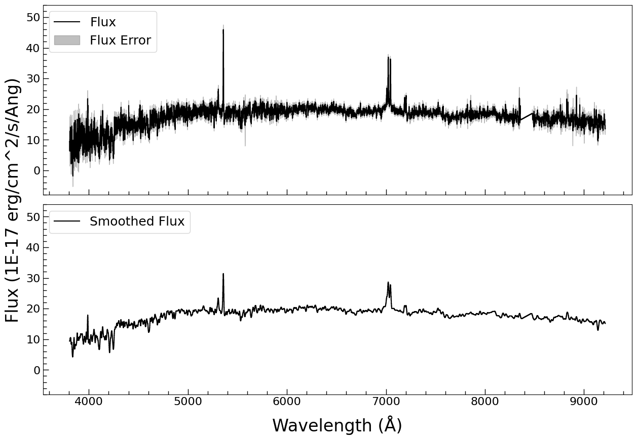
_images/sdss0006_spectrum.png — The spectrum as it arrives, and the same 3-pixel-smoothed. The 4 000 A break is the host galaxy, the two spikes are H-alpha and [O III] 5007: at this redshift the galaxy’s 4000 A break and the AGN’s lines are both inside one SDSS window.#

# %% deredden
import extinction

A_lambda = extinction.ccm89(wave_obs, A_V, r_v=3.1)
wave_rest = wave_obs / (1 + REDSHIFT)
flux_dered = flux_obs * 10**(0.4 * A_lambda)
ferr_dered = ferr_obs * 10**(0.4 * A_lambda)

fig, axs = plt.subplots(2, 1, figsize=(15, 10), sharex=True, sharey=True)
axo = fig.add_subplot(111, frameon=False) # The out axis
axo.tick_params(axis='y', which='both', left=False, labelleft=False)
axo.tick_params(axis='x', which='both', bottom=False, labelbottom=False)
axo.set_ylabel(f'Flux ({units})', fontsize=24, labelpad=30)

ax = axs[0]
ax.step(wave_obs, flux_obs, where='mid', color='C0', alpha=0.5, label='Original Flux')
ax.step(wave_obs, flux_dered, where='mid', color='C3', alpha=0.5, label='Dereddened Flux')
ax.minorticks_on()
ax.set_xlabel(r'Obs. Wavelength (Å)', fontsize=24)
ax.set_ylim(-8, 54)
ax.legend(loc='upper left', fontsize=14, ncols=3)

ax = axs[1]
ax.step(wave_rest, flux_dered, where='mid', color='k', alpha=1, label='Dereddened Flux (Rest Frame)')
ax.minorticks_on()
ax.set_xlabel(r'Rest Wavelength (Å)', fontsize=24)
ax.set_ylim(-8, 54)
ax.legend(loc='upper left', fontsize=14, ncols=3)
plt.show()

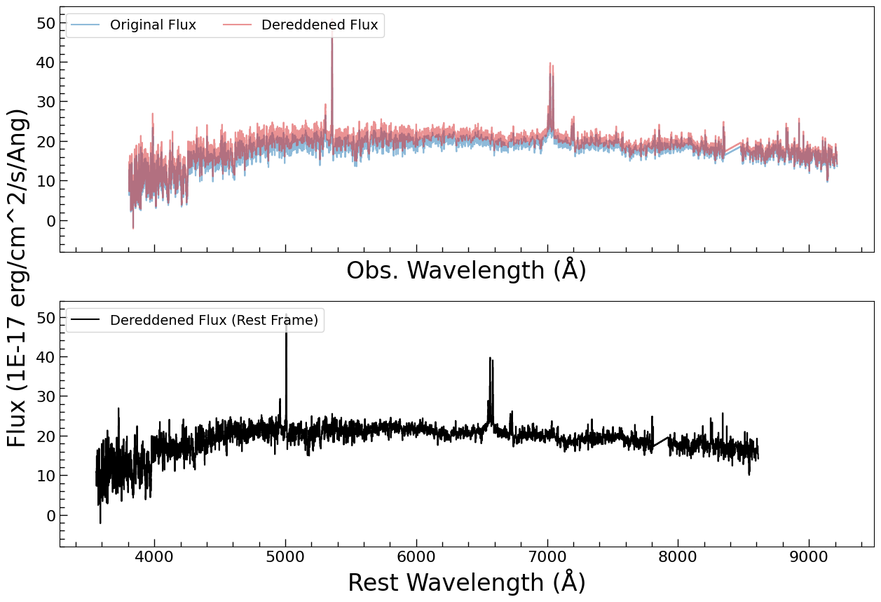
_images/sdss0006_dereddened.png — Top: the observed flux and the same flux with the foreground reddening removed – the correction is a slope, so it lifts the blue end by about 10%. Bottom: the same flux in the rest frame, 3 560-8 610 A – the model is fitted in that frame, so this is the spectrum every stage below sees. The gap at 7 600 A is the dichroic edge, and no window crosses it.#

2. The continuum windows #

The starlight is fitted only where there are no emission lines, because an emission line in the continuum fit would be absorbed by a stellar template’s absorption feature and then subtracted from the data before the lines are measured. The six windows are the ones Greene & Ho (2005) use for this purpose: 3 900-4 060 (which includes Ca II H and K, the sharpest features in the whole spectrum), 4 170-4 260, 4 430-4 770, 5 080-5 550, 6 050-6 200 and 6 890-7 010 A. That is 1 153 of the 3 841 pixels – 30%; the other 70% enter the likelihood with zero weight, through a boolean mask rather than by truncating the arrays.

# %% cont_windows
# From Greene & Ho (2005, ApJ, 630, 122); The first window is to include Ca II K&H.
cont_windows = [[3900, 4060], [4170, 4260], [4430, 4770], [5080, 5550], [6050, 6200], [6890, 7010]]

fig, ax = plt.subplots(1, 1, figsize=(15, 5))
ax.step(wave_rest, gaussian_filter1d(flux_dered, 2), where='mid', color='k', label='Dereddened Flux')
for window in cont_windows:
    ax.axvspan(window[0], window[1], color='C1', alpha=0.5)
ax.set_xlabel(r'Rest Wavelength (Å)', fontsize=24)
ax.set_ylabel(f'Flux ({units})', fontsize=24)
ax.minorticks_on()
ax.set_ylim(-8, 54)
ax.legend(loc='upper left', fontsize=14)
plt.savefig(OUTPUT_DIR / 'sdss0006_continuum_fit.png', dpi=140, bbox_inches='tight')
plt.show()

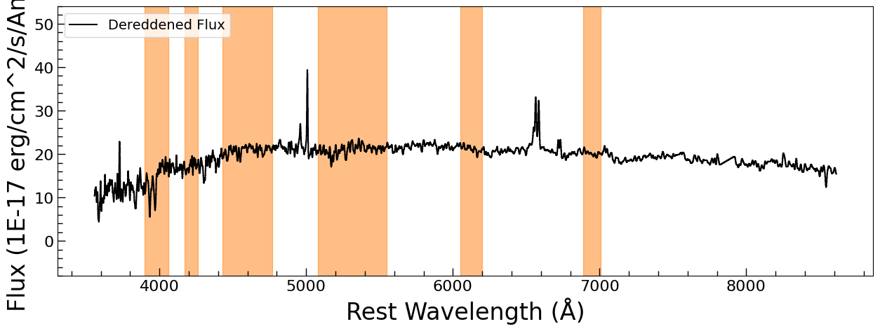
_images/sdss0006_windows.png — The dereddened rest-frame spectrum with the six continuum windows shaded. Note what is *outside* them: H-beta and [O III] 4959/5007, the Mg I b triplet region around 5 170 (inside the fourth window, and a reason it is 470 A wide), H-alpha with [N II] and [S II], and the [S II] 6716/6731 pair.#

3. The continuum model #

Five stellar templates and a power law. The templates are StarSpectrum objects – a population’s spectrum resampled onto a velocity grid and broadened by the galaxy’s velocity dispersion – one per spectral type, A through M, and each carries a free amplitude because the mix of populations is what the data are supposed to decide, not an assumption. One width and one velocity shift are shared by all five: a single galaxy has one sigma_*, and its stars cannot move relative to each other.

# %% model_continuum
# ---- the stellar continuum: five templates, one width and one shift between them -----
velscale = 20                                  # km/s per template pixel
bounds = {'sigma': (velscale, 300)}            # Following Kong & Ho (2018, ApJ, 865, 116)

stars = None
for star_type, amplitude in [('A', 0.81861348), ('F', 9.00857466), ('G', 7.32022514),
                             ('K', 4.28809967), ('M', 3.73763399)]:
    star = jxm.StarSpectrum(amplitude=amplitude, sigma=79.62810518, delta_z=-0.00031473,
                            velscale=velscale, Star_type=star_type, name=f'{star_type} Star',
                            bounds=bounds)
    stars = star if stars is None else stars + star

for mn in ['A Star', 'F Star', 'G Star', 'M Star']:
    stars[mn].sigma.tied = jxm.tie_StarSpectrum_sigma('K Star')
    stars[mn].delta_z.tied = jxm.tie_StarSpectrum_deltaz('K Star')

pl = jxm.PowerLaw1D(amplitude=3.35418096, x_0=5000., alpha=-0.26414091, name='PowerLaw',
                    fixed={'x_0': True, 'alpha': False})
# The iron pseudo-continuum: this object shows no significant iron features, so it is left
# out, exactly as in the reference notebook.
model_cont = stars + pl
print(f"{len(model_cont.submodel_names)} components, "
      f"{len(model_cont.free_param_names)} free parameters: {model_cont.free_param_names}")

Nine free parameters, and they are worth naming: five star amplitudes, one velocity dispersion, one redshift offset, the power law’s amplitude and its slope. The iron pseudo-continuum is left out, and that is a measurement rather than an omission – this object’s spectrum shows no significant Fe II structure, so a template for it would fit noise.

The priors are the part that makes this reproducible on another object, because every one is scaled from the spectrum in the cell that sets it: a star amplitude or a power-law amplitude is a LogUniform from 10^-2 to three times the brightest continuum pixel, the velocity dispersion a Uniform from the velocity scale of the templates (20 km/s) to 300 km/s (following Kong & Ho 2018), the redshift offset a Uniform of +-0.001, and the slope a Uniform of +-2 in F_lambda, which covers every optical AGN slope anyone has measured.

# %% priors_continuum
# ---- one prior per free parameter, scaled from the spectrum -------------------------
# A stellar amplitude and the power-law amplitude are both "a multiple of the continuum":
# any value from invisible to three times the brightest continuum pixel.
use_cont = np.zeros_like(wave_rest, dtype=bool)
for window in cont_windows:
    use_cont |= (wave_rest >= window[0]) & (wave_rest <= window[1])
weights = use_cont.astype(float)

peak_cont = float(np.max(flux_dered[use_cont]))
amp_cont = priors.LogUniform(1e-2, 3.0 * peak_cont)

for mn in ['A Star', 'F Star', 'G Star', 'K Star', 'M Star']:
    model_cont[mn].amplitude.prior = amp_cont
model_cont['PowerLaw'].amplitude.prior = amp_cont
# F_lambda ~ lambda^alpha over 3900-7000 A: every optical AGN slope in the literature is
# inside +-2, and a wider box spends its volume on slopes no AGN has -- which is what pulls
# the 5100 A level low when the slope is left free over +-5.
model_cont['PowerLaw'].alpha.prior = priors.Uniform(-2.0, 2.0)
model_cont['K Star'].sigma.prior = priors.Uniform(velscale, 300.0)
model_cont['K Star'].delta_z.prior = priors.Uniform(-0.001, 0.001)

free = set(model_cont.free_param_names)
pairs = list(zip(model_cont.param_names, model_cont.qualified_param_names))
unset = [q for flat, q in pairs if flat in free and model_cont.get_prior(q) is None]
print(f"{len(free)} free parameters; without a prior: {unset}")
assert not unset

The fit returns the posterior, not a minimum, and the cell prints it as median with 16th and 84th percentiles:

A Star.amplitude          0.16686      0.11      0.25
F Star.amplitude           9.0816      0.68      0.72
G Star.amplitude           10.092      0.67      0.58
K Star.amplitude           1.2311      0.53      0.68
K Star.sigma               74.202       5.3       5.6
K Star.delta_z         -0.00033186     2e-05     2e-05
M Star.amplitude           3.3809      0.63      0.58
PowerLaw.amplitude         3.5424      0.42      0.36
PowerLaw.alpha           -0.70001      0.38      0.28

# %% fit_continuum
started = time.perf_counter()
fit_cont = JNesty_Fit(model_cont, wave_rest[use_cont], flux_dered[use_cont],
                      ferr_dered[use_cont], nlive=nlive, bound='multi', device=DEVICE,
                      queue_size=QUEUE_SIZE)
fit_cont.fit(progress=False, dlogz=dlogz, max_iterations=MAX_ITERATIONS)
print(f"log Z = {fit_cont.log_evidence:.2f} +- {fit_cont.log_evidence_err:.2f}"
      f"   ({fit_cont.n_iterations} iterations, {(time.perf_counter() - started) / 60:.1f} min)")

# The reference prints one `m.__repr__()` per component. With a sampler the answer is a
# posterior per parameter, so the table below holds all of them: median and 16th/84th
# percentiles, which is a 68% credible interval.
lo_cont, med_cont, hi_cont = fit_cont.get_quantiles((0.16, 0.5, 0.84))
print(f"\n  {'parameter':22s} {'median':>10s} {'-':>9s} {'+':>9s}")
print("  " + "-" * 52)
for name, m, l, h in zip(fit_cont.full_param_names, med_cont, lo_cont, hi_cont):
    print(f"  {name:22s} {m:10.5g} {m - l:9.2g} {h - m:9.2g}")

model_cont.set_free_params(med_cont)          # draw the medians, not the last sample

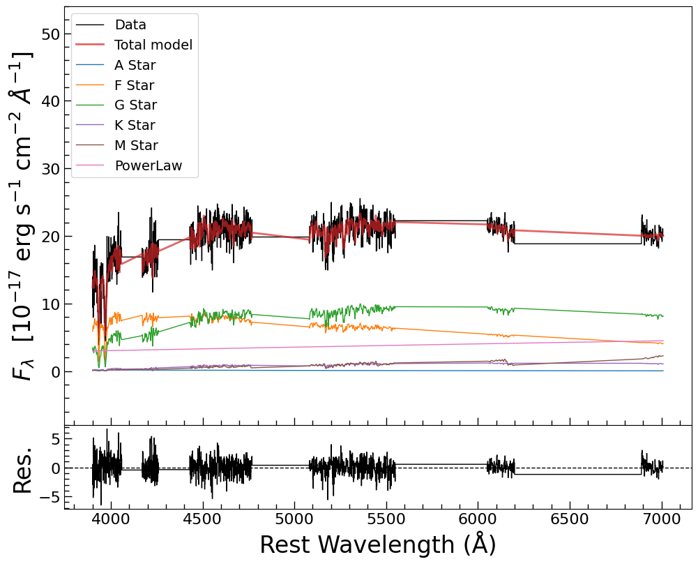
_images/sdss0006_continuum_fit.png — The continuum fit: the six windows, the data, the total model, and the five templates plus the power law underneath it. The lower panel is the residual in units of the error. At 3.2 minutes this is the longest of the four stages – they sum to six – because it is the only one with a strongly degenerate parameter space.#

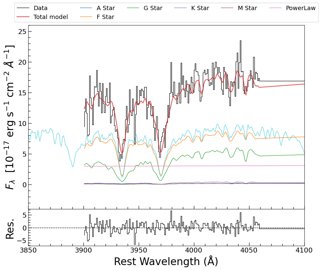
_images/sdss0006_caii.png — Ca II H and K, zoomed. These are the features that measure `sigma_*`. At 3 950 A the SDSS line-spread function is 2.4 A in FWHM, a sigma of 77 km/s: the instrument is as wide as the dispersion being measured, so the fit reads a line that is barely broader than the instrumental profile – which is why the width below is the fragile number.#

4. sigma_* and the 5100 A luminosity #

Two numbers are taken out of the continuum stage. The first is the posterior of K Star.sigma – the shared velocity dispersion, so any of the five stars would give it. The second is the luminosity at 5100 A, and it is not read off the power law’s amplitude: amplitude and slope are correlated, so the level at 5100 A is computed per sample, amp * (5100/5000)**alpha, and the median of that distribution is quoted with its own percentiles. Taking the median of each parameter and multiplying afterwards would not give the same number.

# %% flux_lines
from astropy.cosmology import Planck18 as cosmo

flux_lines = flux_dered - model_cont(wave_rest)
fig, ax = plt.subplots(1, 1, figsize=(15, 5))
ax.step(wave_rest, flux_lines, where='mid', color='k', label='Emission Line Spectrum')
ax.step(wave_rest, gaussian_filter1d(flux_lines, 2), where='mid', lw=1, color='r', label='Smoothed Emission Line Spectrum')
ax.set_xlabel(r'Rest Wavelength (Å)', fontsize=24)
ax.set_ylabel(f'Flux ({units})', fontsize=20)
ax.minorticks_on()
ax.legend(loc='upper left', fontsize=14, ncols=2)
plt.show()

lum_dist = cosmo.luminosity_distance(REDSHIFT).to('cm').value
col_cont = {name: index for index, name in enumerate(fit_cont.param_names)}
samples_cont = np.asarray(fit_cont.samples_equal_weight, dtype=float)

# lambda L_lambda(5100): the reference's m_fit['PowerLaw'].amplitude * 5100 * 1e-17, per sample
lam_rest = 5100.0
lamFlam = (samples_cont[:, col_cont['amplitude_5']]
           * (lam_rest / 5000.0) ** samples_cont[:, col_cont['alpha_5']] * lam_rest * 1e-17)
nuLnu_samples = lamFlam * 4 * np.pi * lum_dist**2               # erg/s

sigma_star = float(np.median(samples_cont[:, col_cont['sigma_3']]))     # km/s
sigma_star_lo, sigma_star_hi = np.percentile(samples_cont[:, col_cont['sigma_3']], [16, 84])
nuLnu = float(np.median(nuLnu_samples))
nuLnu_lo, nuLnu_hi = np.percentile(nuLnu_samples, [16, 84])

print('\nThe velocity dispersion (sigma) is {:.2f} (-{:.2f}/+{:.2f}) km/s'.format(
    sigma_star, sigma_star - sigma_star_lo, sigma_star_hi - sigma_star))
print('The 5100 Å continuum luminosity is {:.2e} (-{:.2e}/+{:.2e}) erg/s'.format(
    nuLnu, nuLnu - nuLnu_lo, nuLnu_hi - nuLnu))

The velocity dispersion (sigma) is 74.20 (-5.27/+5.56) km/s
The 5100 A continuum luminosity is 2.27e+42 (-2.83e+41/+2.38e+41) erg/s

5. What the continuum posterior is, and is not #

The two numbers above do not have the same quality, and the difference is a property of the model rather than of the sampler.

The 5100 A luminosity is robust. Every decomposition in the family of fits carries the same flux at 5100 A – the fit happens 100 A away – so repeated runs give 1.9 to 2.3 x 10^42 erg/s where the interval from one run is +-0.25.

The velocity dispersion is not. The continuum is nine parameters describing one smooth curve, and the split between the five stellar templates and the power law is a direction the data weakly constrain: run the same stage with the same priors and a different sampler bounding (bound='multi' against bound='single') and the evidences agree to 1.3 nats while sigma_* comes out 74.2 and 86.3 km/s – intervals that do not overlap. Both runs are converged approximations of one posterior that neither of them fully mapped. Two consequences, both used below:

the 68% interval from one run (+-5 km/s) is narrower than the run-to-run spread, so sigma_* = 74 +- 10 km/s is the error to carry into the M-sigma panel;
the decomposition itself – which star is bright, what the slope is – is not a measurement. The K star’s amplitude is 1.2 in this run and was 4.3 in the least-squares fit of the same windows, and the power-law slope is -0.70 here against -0.26 there: the two fits trade starlight for power law and still land on the same flux at 5100 A.

That is worth internalising before using any staged continuum decomposition: a least-squares fit would have returned one of those decompositions as the answer, with an error bar from the covariance matrix that is just as optimistic.

6. The narrow-line template, measured on [S II]#

Every narrow line in the rest of the analysis is one measured profile with an amplitude each, rather than a Gaussian with a width each. The profile is measured here, on [S II] 6716/6731: the two peaks give two samplings of the same shape, and apart from one unmodelled spike at 6 762 A the 100 A window is clean.

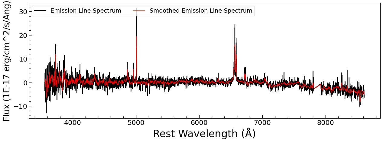
_images/sdss0006_line_spectrum.png — The spectrum with the best-fit continuum subtracted – what stages 2 to 4 have to explain. H-beta and [O III], H-alpha with [N II] and [S II], the [O I] pair at 6 300/6 364, and little else: the red end is clean, which is why [S II] can be measured on its own first.#

The model is a Line_MultiGauss_doublet with one core and one wind per peak – the wind is the broad base that a Gaussian cannot bend into, and it is what makes the profile worth measuring rather than assuming. Seven free parameters: two amplitudes, one shared width, one shared shift, and the wind’s three (relative amplitude, shift, width).

# %% model_sii
window = [6680, 6780]
fltr = (wave_rest > window[0]) & (wave_rest < window[1])
wave_sii = wave_rest[fltr]
flux_sii = flux_lines[fltr]
ferr_sii = ferr_dered[fltr]

cont_sii = jxm.PowerLaw1D(amplitude=0, x_0=6730., alpha=0,
                          fixed=dict(x_0=True, alpha=True, amplitude=True), name='Cont SII')
sii = jxm.Line_MultiGauss_doublet(n_components=2, amp_c0=6.12614425, amp_c1=5.85356985,
                                  dv_c=93.05894619, sigma_c=105.07513204,
                                  amp_w0=0.1, dv_w0=0, sigma_w0=200,
                                  wavec0=wavec_sii_6716, wavec1=wavec_sii_6731, name='[SII]')
model_sii = cont_sii + sii
print(f"{len(model_sii.free_param_names)} free parameters: {model_sii.free_param_names}")

# %% priors_sii
# ---- one prior per free parameter, scaled from the window ---------------------------
peak_sii = float(np.max(flux_sii))
sii.amp_c0.prior = priors.LogUniform(0.1, 3.0 * peak_sii)    # [S II] 6716
sii.amp_c1.prior = priors.LogUniform(0.1, 3.0 * peak_sii)    # [S II] 6731 (a ratio, but free:
                                                             # this is the density diagnostic)
sii.dv_c.prior = priors.Uniform(-1000.0, 1000.0)             # km/s
sii.sigma_c.prior = priors.Uniform(20.0, 300.0)              # km/s: resolved to very broad
sii.amp_w0.prior = priors.Uniform(1e-3, 1.0)                 # the wing, as a ratio to the core
sii.dv_w0.prior = priors.Uniform(-1000.0, 1000.0)
sii.sigma_w0.prior = priors.Uniform(20.0, 300.0)

free = set(model_sii.free_param_names)
pairs = list(zip(model_sii.param_names, model_sii.qualified_param_names))
unset = [q for flat, q in pairs if flat in free and model_sii.get_prior(q) is None]
print(f"{len(free)} free parameters; without a prior: {unset}")
assert not unset

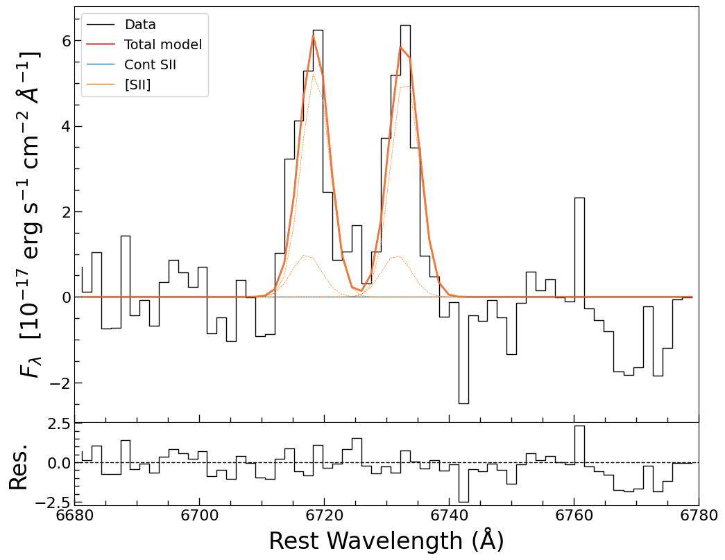
_images/sdss0006_sii_fit.png — The [S II] fit, `log Z = -94.58 +- 0.08` in 0.5 minutes. The solid curves are the two peaks, the dotted ones the winds. The spike at 6 762 A is real in the data and absent from the model: it is 1 500 km/s from 6731, outside both profiles, so the ratio of the two peaks is unaffected – at the price of a handful of large residuals.#

The template is then read off the model – gen_template returns the single-line profile on a velocity grid, centred and normalised – and written out with its provenance. It is this file, not the model, that the next two stages use, and that is what makes the four stages independent.

# %% template
# Generate the narrow line template: the fitted doublet's *single-line* profile in velocity
# space, unit peak.  gen_template reads the current parameters, and the medians are on the
# model since the fit cell above, so this is the measured profile -- not a Gaussian.
ls_km = galspec.constants.ls_km

velc_temp = np.arange(-3e3, 3e3, 5)
flux_temp = np.asarray(model_sii['[SII]'].gen_template(velc_temp))
temp_data = np.array([velc_temp, flux_temp]).T
np.savetxt(OUTPUT_DIR / 'sdss0006_sii_template.txt', temp_data, fmt='%5e')

half = np.where(flux_temp >= 0.5)[0]
print(f"template: {flux_temp.size} velocity bins, peak {flux_temp.max():.3f}, "
      f"FWHM {velc_temp[half[-1]] - velc_temp[half[0]]:.0f} km/s")
print(f"  wrote {OUTPUT_DIR / 'sdss0006_sii_template.txt'}")

fig, ax = plt.subplots(figsize=(7, 7))
ax.plot(velc_temp, flux_temp)
ax.axhline(0.5, color='0.7', lw=0.8, ls=':')
ax.set_xlabel('Velocity (km/s)', fontsize=16)
ax.set_ylabel('Normalised flux', fontsize=16)
ax.minorticks_on()
plt.savefig(OUTPUT_DIR / 'sdss0006_sii_template_profile.png', dpi=140, bbox_inches='tight')
plt.show()

template: 1200 velocity bins, peak 1.000, FWHM 240 km/s

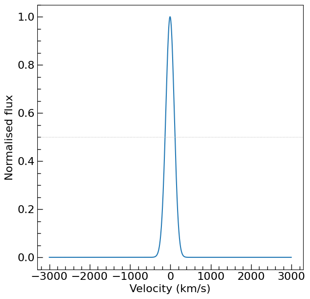
_images/sdss0006_sii_template.png — The measured profile: FWHM 240 km/s, with the wings the wind accounts for. The reference least-squares fit of the same spectrum gives 245 km/s.#

7. The H-alpha complex #

The continuum-subtracted spectrum is now fitted in the H-alpha window with four components: broad H-alpha (a Gaussian – the broad-line region does not share the narrow kinematics), narrow H-alpha (the template), and the two narrow doublets [N II] 6548/6583 and [S II] 6716/6731. The doublets are single Line_template_doublet components rather than two templates tied together, so the pair cannot drift apart, and the [N II] ratio is tied to its atomic 2.96 while the [S II] ratio is left free – 6716/6731 is the density diagnostic, and this fit measures 1.04, which is the low-density end.

# %% model_ha
window = [6400, 6900]
fltr = (wave_rest > window[0]) & (wave_rest < window[1])
wave_ha = wave_rest[fltr]
flux_ha = flux_lines[fltr]
ferr_ha = ferr_dered[fltr]

bha = jxm.Line_MultiGauss(n_components=1, amp_c=4.03952323, dv_c=150.30995833,
                          sigma_c=1102.23008001, wavec=wavec_ha, name='bHalpha')
nha = jxm.Line_template(template_velc=velc_temp, template_flux=flux_temp,
                        amplitude=16.99272669, dv=86.18868006, wavec=wavec_ha, name='nHalpha')
# The two narrow doublets: one template doublet each, so the shared shift is structural and
# the pair cannot drift apart.  line.single(wave, comp) then gives one line of it.
nii = jxm.Line_template_doublet(template_velc=velc_temp, template_flux=flux_temp,
                                amp_c0=16.55604126, amp_c1=16.55604126 / 2.96, dv_c=0,
                                wavec0=wavec_nii_6583, wavec1=wavec_nii_6548, name='NII')
sii = jxm.Line_template_doublet(template_velc=velc_temp, template_flux=flux_temp,
                                amp_c0=5.23636479, amp_c1=5.65680966, dv_c=0,
                                wavec0=wavec_sii_6716, wavec1=wavec_sii_6731, name='SII')

model_ha = bha + nha + nii + sii

# Tie the parameters: one velocity for every narrow line, and the [N II] doublet ratio
for ln in ['NII', 'SII']:
    model_ha[ln].dv_c.tied = jxm.tie.tie_template_dv('nHalpha')

model_ha['NII'].amp_c1.tied = jxm.tie.tie_MultiGauss_doublet_ratio('NII', ratio=2.96)
# ([S II] 6716/6731 is a density diagnostic, not an atomic ratio: it stays free)

print(f"{len(model_ha.free_param_names)} free parameters: {model_ha.free_param_names}")

# %% priors_ha
# ---- one prior per free parameter, scaled from the window ---------------------------
peak_ha = float(np.max(flux_ha))
bha.amp_c.prior = priors.LogUniform(0.1, 3.0 * peak_ha)
bha.dv_c.prior = priors.Uniform(-1000.0, 1000.0)        # km/s
bha.sigma_c.prior = priors.Uniform(300.0, 6000.0)       # km/s: broader than any narrow line
nha.amplitude.prior = priors.LogUniform(0.1, 3.0 * peak_ha)
nha.dv.prior = priors.Uniform(-500.0, 500.0)            # the systemic velocity, all narrow lines
nii.amp_c0.prior = priors.LogUniform(0.1, 3.0 * peak_ha)
sii.amp_c0.prior = priors.LogUniform(0.1, 3.0 * peak_ha)
sii.amp_c1.prior = priors.LogUniform(0.1, 3.0 * peak_ha)    # the ratio is measured, not fixed
# (the parameters that are tied in the cell above take no prior: their value never comes
# from the prior, and galspec raises if one is set)

free = set(model_ha.free_param_names)
pairs = list(zip(model_ha.param_names, model_ha.qualified_param_names))
unset = [q for flat, q in pairs if flat in free and model_ha.get_prior(q) is None]
print(f"{len(free)} free parameters; without a prior: {unset}")
assert not unset

Eight free parameters, and the prior cell is where the model’s assumptions become visible: the broad line’s width is allowed to reach 6 000 km/s while its shift is confined to +-1 000 km/s around the systemic velocity; every amplitude is LogUniform(0.1, 3 * peak), i.e. from a tenth of the flux unit to three times the window’s peak; and the systemic shift is +-500 km/s, which is wide enough to hold any rotation the template does not know about.

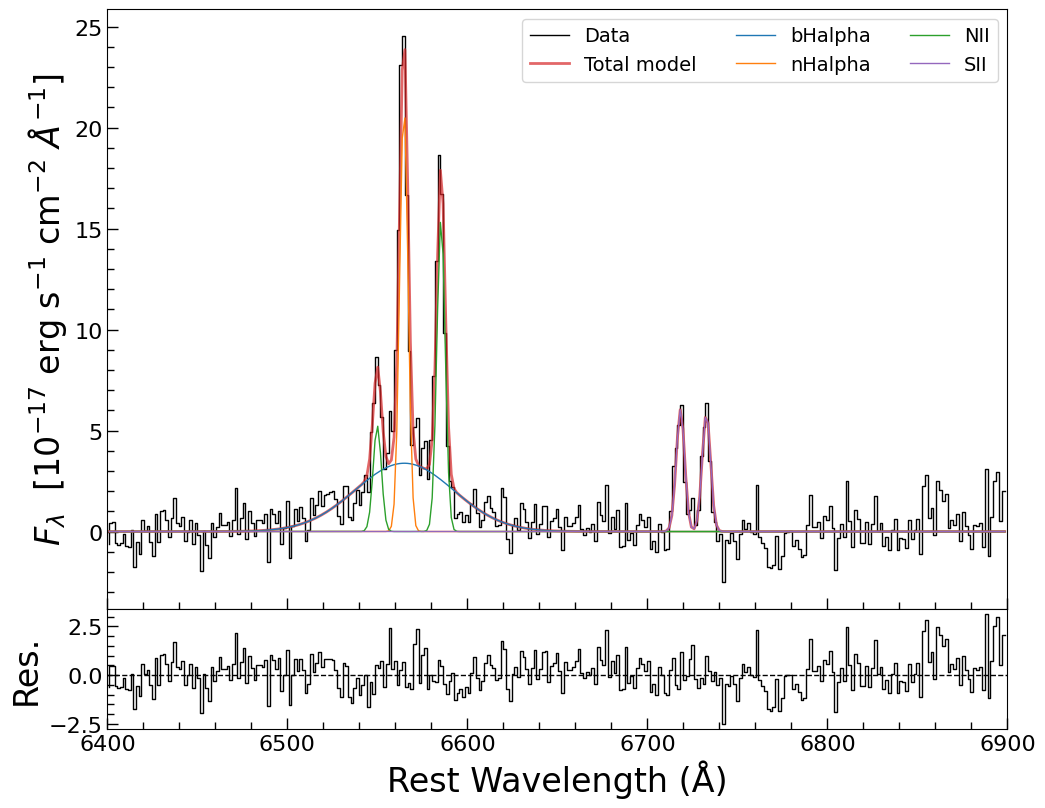
_images/sdss0006_halpha_fit.png — The H-alpha window, `log Z = -454.60 +- 0.11` in 0.9 minutes. Broad H-alpha under the two [N II] lines, and the [S II] pair on the right, each doublet drawn as one curve.#

bHalpha.amp_c               3.3818      0.27      0.29
bHalpha.dv_c               96.659        78        76
bHalpha.sigma_c            1247.9   1.1e+02   1.2e+02
nHalpha.amplitude          21.146      0.73      0.73
nHalpha.dv                 94.851       2.8       2.8
NII.amp_c0                 15.526      0.62      0.63
SII.amp_c0                 6.0437      0.53      0.54
SII.amp_c1                 5.8324      0.53      0.54

The narrow H-alpha shift of 94.9 +- 2.8 km/s is the systemic velocity, and it is the one dv that every other narrow line inherits from here on – H-beta, [O III] and the [O III] wing are all tied to it, which is what “the narrow-line region moves as one body” means in a model.

8. H-beta and [O III]#

The second window pair – 4 700-5 100 and 6 400-6 900 A – brings H-beta, the [O III] doublet and a broad wing under [O III] 5007. The fit is now over both windows at once with the H-alpha complex carried along unchanged, so the narrow lines keep one velocity across a 1 700 A baseline. H-beta shares broad H-alpha’s shift but not its width: the width is a measurement, and it is the one that goes into the black-hole mass.

# %% model_hb
window_list = [[4700, 5100], [6400, 6900]]
fltr = np.zeros_like(wave_rest, dtype=bool)
for window in window_list:
    fltr |= (wave_rest > window[0]) & (wave_rest < window[1])
wave_hb = wave_rest[fltr]
flux_hb = flux_lines[fltr]
ferr_hb = ferr_dered[fltr]

bhb = jxm.Line_MultiGauss(n_components=1, amp_c=3.29861897, dv_c=98.83475277,
                          sigma_c=1272.70115266, wavec=wavec_hb, name='bHbeta')
nhb = jxm.Line_template(template_velc=velc_temp, template_flux=flux_temp,
                        amplitude=16.99272669, dv=86.18868006, wavec=wavec_hb, name='nHbeta')
# the [O III] doublet, one template doublet with the atomic ratio imposed below
oiii = jxm.Line_template_doublet(template_velc=velc_temp, template_flux=flux_temp,
                                 amp_c0=16.55604126, amp_c1=16.55604126 / 2.98, dv_c=0,
                                 wavec0=wavec_oiii_5007, wavec1=wavec_oiii_4959, name='OIII')
# the broad [O III] wing: a Gaussian at each peak of the doublet
no3_w = jxm.Line_MultiGauss_doublet(n_components=1, amp_c0=3.0, amp_c1=3.0/2.98, dv_c=0,
                                    sigma_c=300, wavec0=wavec_oiii_5007,
                                    wavec1=wavec_oiii_4959, name='OIII_w')

model_hb = bhb + nhb + oiii + no3_w + model_ha     # the fitted H-alpha complex comes along

# Tie the parameters
model_hb['nHbeta'].dv.tied = jxm.tie.tie_template_dv('nHalpha')
model_hb['OIII'].dv_c.tied = jxm.tie.tie_template_dv('nHalpha')
model_hb['OIII'].amp_c1.tied = jxm.tie.tie_MultiGauss_doublet_ratio('OIII', ratio=2.98)
model_hb['OIII_w'].amp_c1.tied = jxm.tie.tie_MultiGauss_doublet_ratio('OIII_w', ratio=2.98)
model_hb['OIII_w'].dv_c.tied = jxm.tie.tie_template_dv('nHalpha')
model_hb['bHbeta'].dv_c.tied = jxm.tie.tie_MultiGauss_dv_c('bHalpha')

print(f"{len(model_hb.free_param_names)} free parameters: {model_hb.free_param_names}")

# %% priors_hb
# ---- one prior per free parameter, scaled from the two windows ----------------------
peak_hb = float(np.max(flux_hb))
bhb.amp_c.prior = priors.LogUniform(0.1, 3.0 * peak_hb)
bhb.sigma_c.prior = priors.Uniform(300.0, 6000.0)       # km/s
nhb.amplitude.prior = priors.LogUniform(0.1, 3.0 * peak_hb)
oiii.amp_c0.prior = priors.LogUniform(0.1, 3.0 * peak_hb)
# The wing stops at half the peak (see the note above this cell): it sits at the same
# wavelength as the template, so a wing free to reach the line's strength can absorb the line.
no3_w.amp_c0.prior = priors.LogUniform(0.1, 0.5 * peak_hb)   # a broad base, not the line
no3_w.sigma_c.prior = priors.Uniform(30.0, 2000.0)      # km/s: a wing, not a line core
# (the parameters that are tied in the cell above take no prior: their value never comes
# from the prior, and galspec raises if one is set)

free = set(model_hb.free_param_names)
pairs = list(zip(model_hb.param_names, model_hb.qualified_param_names))
unset = [q for flat, q in pairs if flat in free and model_hb.get_prior(q) is None]
print(f"{len(free)} free parameters; without a prior: {unset}")
assert not unset

Two priors deserve a note. The broad [O III] wing’s amplitude is bounded to half the window’s peak, because the wing sits at the same wavelength as the [O III] template: leave it free to reach the line’s strength and the sampler finds the decomposition in which the “wing” is the line – amplitude 30 where 0.4 belongs, a starved narrow line under it, and an [O III] flux two orders of magnitude low. Bounding the wing is a prior choice, not a measurement, and it is the one choice on this page that changes a number if it is made differently. The wing’s width runs up to 2 000 km/s for the opposite reason: a wing is not a line core, and nothing in the data says how far its tail goes.

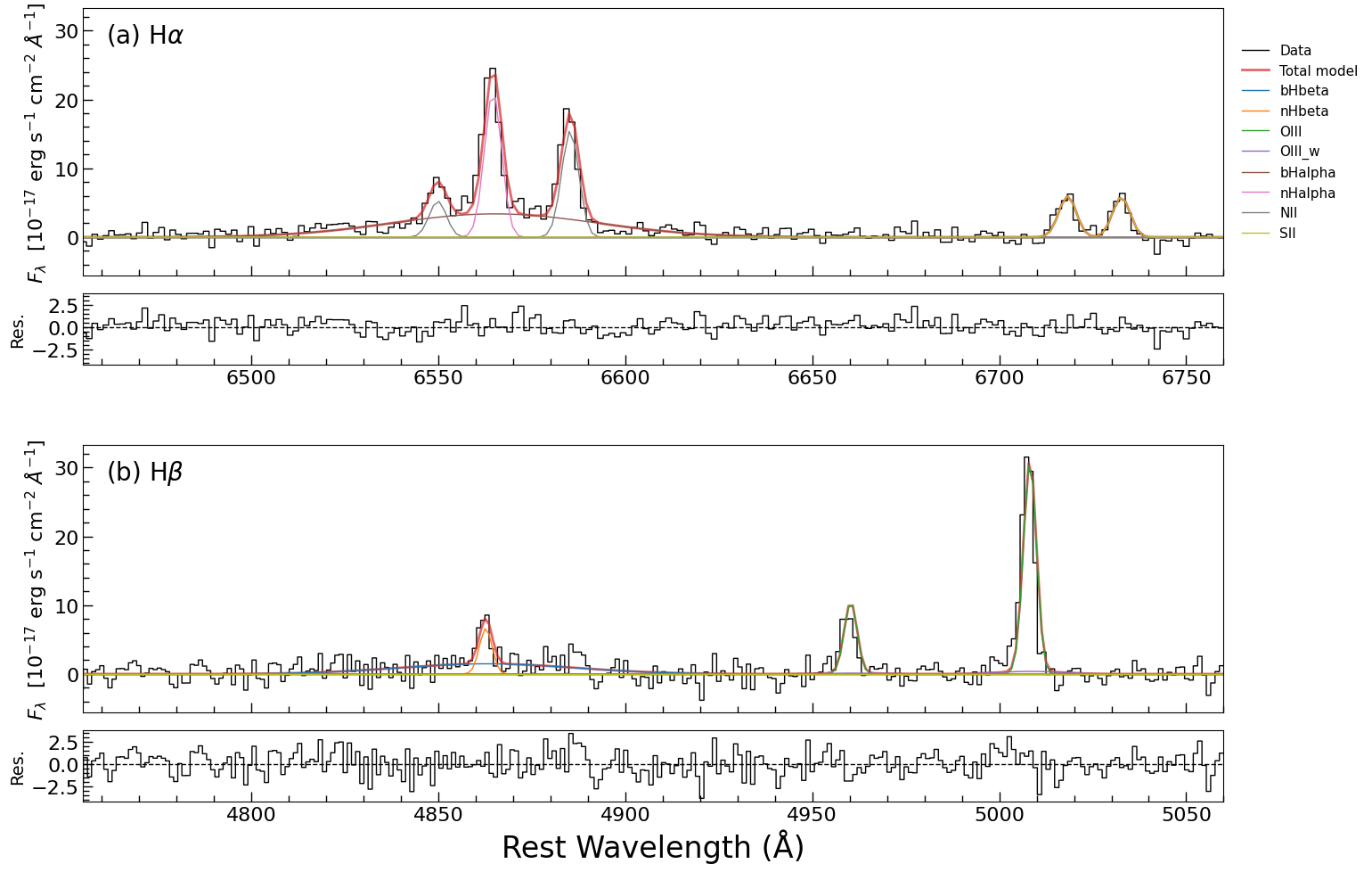
_images/sdss0006_hbeta_halpha.png — Both windows from the final stage, `log Z = -1070.14 +- 0.14` in 1.5 minutes: (a) the H-alpha complex, (b) H-beta, [O III] 4959/5007 and the broad base under 5007. The [O III] pair is one doublet with the atomic 2.98 ratio imposed; the lowest panel is the residual.#

bHbeta.amp_c               1.4843      0.27      0.28
bHbeta.sigma_c             1457.8   2.5e+02     3e+02
nHbeta.amplitude           6.6369      0.86      0.86
OIII.amp_c0                30.838       1.2         1
OIII_w.amp_c0             0.37986      0.22      0.66
OIII_w.sigma_c              508.4   2.5e+02   6.1e+02

The [O III] wing is detected but not measured: an amplitude of 0.38 (-0.22/+0.66) and a width of 510 (-250/+610) km/s say that something broad is under 5007 and that neither its strength nor its shape is pinned down. Do not read a velocity off it.

9. The fluxes and the widths #

Line fluxes are combinations of parameters, so they are computed per posterior sample rather than from the medians – that is how the error bar inherits the correlations in the fit – and for a doublet, one line at a time: Line_template_doublet.single(wave, comp) gives the profile of one line of a pair, which is what [N II] 6583, [O III] 5007 and each [S II] line need. Integrating a doublet whole would fold 6548 into the [N II] flux.

# %% physical_parameters
def integrate_line_flux(model, line_name, wave_obs, theta, scale=1e-17, comp=None):
    """
    Integrate the line flux from the fitted model.

    Parameters:
    model : JaxModel
        The fitted model containing the emission line.
    line_name : str
        The name of the emission line to integrate.
    wave_obs : array-like
        Very important! We should use the observed wavelength array.
    theta : array-like
        One posterior sample: the free parameters of the model.
    scale : float, optional
        The scale factor to convert the flux units, default is 1e-17 erg/s/cm^2/Å.
    comp : int, optional
        For a doublet, which line to take: 0 for the line at ``wavec0``, 1 for the
        one at ``wavec1``.  ``None`` (the default) integrates everything under
        ``line_name``, which for a doublet is both peaks.

    Returns:
    line_flux : float
        The integrated line flux in erg/s/cm^2.
    """
    model.set_free_params(theta)                     # ties are resolved here
    line = model[line_name]
    flux = line(wave_obs) if comp is None else line.single(wave_obs, comp)
    return np.trapezoid(np.asarray(flux) * scale, wave_obs)


def cal_fwhm(model, line_name, theta, vlim=10000, comp=None):
    """
    Calculate the FWHM of the emission line from the fitted model.
    This function allows for complex line profiles.

    Parameters:
    model : JaxModel
        The fitted model containing the emission line.
    line_name : str
        The name of the emission line to calculate FWHM.
    theta : array-like
        One posterior sample: the free parameters of the model.
    comp : int, optional
        For a doublet, which line to measure.  ``None`` measures the first line of
        a doublet (the width of both peaks together is not a line width).

    Returns:
    fwhm : float
        The FWHM of the emission line in km/s.
    """
    model.set_free_params(theta)
    line = model[line_name]
    if comp is None and 'wavec' not in line.param_names:
        comp = 0                                     # a doublet: measure it line by line
    centre = float(line.wavec.value) if comp is None else \
        float(line.wavec0.value if comp == 0 else line.wavec1.value)
    velc = np.linspace(-vlim, vlim, 10000)
    wave = (1 + velc / ls_km) * centre
    flux = np.asarray(line(wave) if comp is None else line.single(wave, comp))
    half_max = np.max(flux) / 2
    indices = np.where(flux >= half_max)[0]
    return velc[indices[-1]] - velc[indices[0]]


samples_hb = np.asarray(fit_hb.samples_equal_weight, dtype=float)

# A flux and a width are evaluations of the model, and the posterior has one entry per dead
# point -- tens of thousands of them.  Two thousand draws resolve a 16th/84th percentile to
# well under a percent and take seconds instead of minutes, so the tail is thinned here.
# (The percentile error of a 2000-draw quantile is sqrt(p(1-p)/n) ~ 0.9%.)
step = max(1, samples_hb.shape[0] // 2000)
samples_hb = samples_hb[::step]

# Each quantity names the model component it comes from, and for a doublet which line of it:
# a BPT diagram wants [N II] 6583, not 6583+6548, and both [S II] lines for the ratio.
LINE_SPECS = [('bHbeta', 'bHbeta', None),
              ('bHalpha', 'bHalpha', None),
              ('nHbeta', 'nHbeta', None),
              ('nHalpha', 'nHalpha', None),
              ('OIII_5007', 'OIII', 0),
              ('NII_6583', 'NII', 0),
              ('SII_6716', 'SII', 0),
              ('SII_6731', 'SII', 1)]
print(f"fluxes and widths from {samples_hb.shape[0]} of the posterior samples")

# the posterior (the reference reads these off one best-fit model)
line_flux = {key: np.array([integrate_line_flux(model_hb, name, wave_obs, theta, comp=comp)
                            for theta in samples_hb])
             for key, name, comp in LINE_SPECS}
line_flux['SII'] = line_flux['SII_6716'] + line_flux['SII_6731']
fwhm_ha = np.array([cal_fwhm(model_hb, 'bHalpha', theta) for theta in samples_hb])
fwhm_hb = np.array([cal_fwhm(model_hb, 'bHbeta', theta) for theta in samples_hb])
fwhm_narrow = np.array([cal_fwhm(model_hb, 'OIII', theta, comp=0) for theta in samples_hb])

# The broad and the narrow Balmer lines are kept apart: the black-hole mass wants the broad
# width, the BPT diagram wants narrow-line ratios, and a Balmer decrement means one or the
# other -- never their sum.
flux_bhb = line_flux['bHbeta']
flux_bha = line_flux['bHalpha']
flux_nhb = line_flux['nHbeta']
flux_nha = line_flux['nHalpha']
flux_o3 = line_flux['OIII_5007']
flux_n2 = line_flux['NII_6583']
flux_s2 = line_flux['SII']

# Calculate the BH mass.  nuLnu comes from the continuum stage and fwhm_hb from this one; the
# two posteriors are independent fits, so the pairs below are drawn at random and the quoted
# error carries both stages -- it does not carry any correlation between them, which a staged
# fit cannot see.
rng = np.random.default_rng(0)
logMbh = np.log10((fwhm_hb / 1000)**2 * (nuLnu_samples[rng.integers(0, nuLnu_samples.size, fwhm_hb.size)] / 1e44)**0.533) + 6.91  # Equation (2) of Liu et al. (2019, ApJS, 243, 21)


def line_summary(values):
    lo, med, hi = np.percentile(values, [16, 50, 84])
    return f"{med:12.4g}  -{med - lo:.3g}/+{hi - med:.3g}"


print(f"  {'quantity':22s} {'value':>12s}  68% interval   (flux: erg/s/cm2, width: km/s)")
print("  " + "-" * 80)
for name, values in [('F(H-beta) broad', flux_bhb),
                     ('F(H-alpha) broad', flux_bha),
                     ('F(H-beta) narrow', flux_nhb),
                     ('F(H-alpha) narrow', flux_nha),
                     ('F([O III] 5007)', flux_o3),
                     ('F([N II] 6583)', flux_n2),
                     ('F([S II] 6716+6731)', flux_s2),
                     ('FWHM(H-alpha) broad', fwhm_ha),
                     ('FWHM(H-beta) broad', fwhm_hb),
                     ('log M_BH [M_sun]', logMbh)]:
    print(f"  {name:22s} {line_summary(values)}")
print(f"  {'FWHM([O III]) [km/s]':22s} {np.median(fwhm_narrow):12.0f}"
      "  (the template's shape: no width is fitted)")

F(H-beta) broad           8.772e-16  -1.48e-16/+1.54e-16
F(H-alpha) broad          2.315e-15  -1.28e-16/+1.39e-16
F(H-beta) narrow          2.821e-16  -3.76e-17/+3.58e-17
F(H-alpha) narrow         1.215e-15  -4.11e-17/+4.19e-17
F([O III] 5007)           1.354e-15  -5.52e-17/+4.6e-17
F([N II] 6583)            8.951e-16  -3.46e-17/+3.6e-17
F([S II] 6716+6731)       6.951e-16  -4.71e-17/+4.53e-17
FWHM(H-alpha) broad            2946  -254/+300
FWHM(H-beta) broad             3430  -624/+716
FWHM([O III]) [km/s]            244  (the template's shape: no width is fitted)

The broad and the narrow Balmer fluxes are kept apart on purpose, and the reason is in the two numbers below: the narrow lines give H-alpha/H-beta = 4.3, which is what a reddened narrow-line region looks like (case B is 2.86, and 4.3 is E(B-V) ~ 0.4 on the Galactic extinction curve), while the broad lines give 2.6, i.e. case B within the errors – the broad-line region is behind less dust. (The foreground reddening was removed at the start of the page; this is dust in the galaxy.) Adding the two components together would produce one meaningless average.

10. The BPT diagram #

Two ratios of forbidden to recombination lines, both measured off the model: [N II] 6583 over H-alpha and [O III] 5007 over H-beta. The forbidden lines come from the narrow-line region only, so the Balmer denominator is the narrow component too, in this notebook and in the reference it follows. That is worth spelling out because the other choice is tempting and plausible: the broad Balmer flux is the brighter number, and H-beta is what the black-hole mass uses, so it reads like the natural one to put underneath. It is not – the broad lines are gas at a different radius – and dividing by them dilutes both ratios until the star lands between the demarcation lines, in the “composite” region, which is the wrong answer for a Seyfert 1.

# %% bpt
from astropy.table import Table
from astropy.io import fits
import warnings
from astropy.units import UnitsWarning

warnings.filterwarnings('ignore', category=UnitsWarning)
warnings.filterwarnings('ignore', category=fits.verify.VerifyWarning)
tb = Table.read(TABLE_DIR / 'Liu2019.fits', format='fits')

logLha_l19 = tb['logNHa']
logLhb_l19 = tb['logNHb']
logLn2_l19 = tb['log6583']
logLo3_l19 = tb['log5007']
logLs2_l19 = np.log10(10**tb['log6716'] + 10**tb['log6731'])

fig, axs = plt.subplots(1, 2, figsize=(14, 7), sharex=True, sharey=True)
fig.subplots_adjust(wspace=0.05)

# Narrow-line ratios: [N II], [S II] and [O III] are forbidden, i.e. they come from the
# narrow-line region and not from the broad one, so the Balmer denominator is the narrow
# component too. (See the note above this cell: dividing by the broad flux instead dilutes
# both ratios and parks this Seyfert 1 between the demarcation lines.)
ln2_ha = np.log10(flux_n2 / flux_nha)
lo3_hb = np.log10(flux_o3 / flux_nhb)
ls2_ha = np.log10(flux_s2 / flux_nha)

ax = axs[0]
x_t = np.median(ln2_ha)
y_t = np.median(lo3_hb)
x_t_e = np.percentile(ln2_ha, [16, 84])
y_t_e = np.percentile(lo3_hb, [16, 84])
ax.errorbar(x_t, y_t, xerr=[[x_t - x_t_e[0]], [x_t_e[1] - x_t]], yerr=[[y_t - y_t_e[0]], [y_t_e[1] - y_t]],
            ms=18, marker='*', ls='none', color='C1', mec='k', mew=2, label='This work', zorder=5, capsize=3)

x = logLn2_l19 - logLha_l19
y = logLo3_l19 - logLhb_l19
fltr = ((x > -10) & (x < 10)) & ((y > -10) & (y < 10))
ax.plot(x[fltr], y[fltr], ms=1, marker='.', ls='none', color='k', alpha=0.3)

ax.set_xlabel(r'$\log (L_{\rm [NII]6583}/L_{\rm H\alpha})$', fontsize=20)
ax.set_ylabel(r'$\log (L_{\rm [OIII]5007}/L_{\rm H\beta})$', fontsize=20)
ax.set_xlim(-1.5, 0.8)
ax.set_ylim(-0.8, 2.2)
ax.minorticks_on()

ax = axs[1]
x2_t = np.median(ls2_ha)
x2_t_e = np.percentile(ls2_ha, [16, 84])
ax.errorbar(x2_t, y_t, xerr=[[x2_t - x2_t_e[0]], [x2_t_e[1] - x2_t]], yerr=[[y_t - y_t_e[0]], [y_t_e[1] - y_t]],
            ms=18, marker='*', ls='none', color='C1', mec='k', mew=2, zorder=5, capsize=3)

x = logLs2_l19 - logLha_l19
fltr = ((x > -10) & (x < 10)) & ((y > -10) & (y < 10))
ax.plot(x[fltr], y[fltr], ms=1, marker='.', ls='none', color='k', alpha=0.3)
ax.set_xlabel(r'$\log (L_{\rm [SII]}/L_{\rm H\alpha})$', fontsize=20)
ax.minorticks_on()

# Demarcation lines; Kewley et al. (2001, 2006), Kauffmann et al. (2003)
x1 = np.linspace(-1.5, 0.3, 100)
y1 = 0.61 / (x1 - 0.47) + 1.19
axs[0].plot(x1, y1, ls='-', color='k', lw=2, label='Kewley+2001')

x2 = np.linspace(-1.5, 0.0, 100)
y2 = 0.61 / (x2 - 0.05) + 1.3
axs[0].plot(x2, y2, ls='--', color='k', lw=2, label='Kauffmann+2003')

x3 = np.linspace(-1.5, 0.3, 100)
y3 = 0.72 / (x3 - 0.32) + 1.3
axs[1].plot(x3, y3, ls='-', color='k', lw=2, label='Kewley+2006')

x4 = np.linspace(-0.31, 0.8, 100)
y4 = 1.89 * x4 + 0.76
axs[1].plot(x4, y4, ls='-', color='k', lw=2)

axs[0].legend(loc='upper left', fontsize=14)
axs[1].legend(loc='upper left', fontsize=14)
fig.savefig(OUTPUT_DIR / 'sdss0006_bpt.png', dpi=140, bbox_inches='tight')
plt.show()

print(f"  log([N II] 6583 / H-alpha, narrow) = {x_t:+.3f}  ({x_t_e[0]:+.3f}, {x_t_e[1]:+.3f})")
print(f"  log([O III] 5007 / H-beta, narrow) = {y_t:+.3f}  ({y_t_e[0]:+.3f}, {y_t_e[1]:+.3f})")
print(f"  log([S II] 6716+6731 / H-alpha)    = {x2_t:+.3f}  ({x2_t_e[0]:+.3f}, {x2_t_e[1]:+.3f})")
print(f"  the demarcations at this x: Kewley+2001 {0.61 / (x_t - 0.47) + 1.19:+.2f},"
      f"  Kauffmann+2003 {0.61 / (x_t - 0.05) + 1.3:+.2f}")

log([N II] 6583 / H-alpha, narrow) = -0.133  (-0.152, -0.112)
log([O III] 5007 / H-beta, narrow) = +0.682  (+0.624, +0.745)
log([S II] 6716+6731 / H-alpha)    = -0.242  (-0.276, -0.212)
the demarcations at this x: Kewley+2001 +0.18,  Kauffmann+2003 -2.03

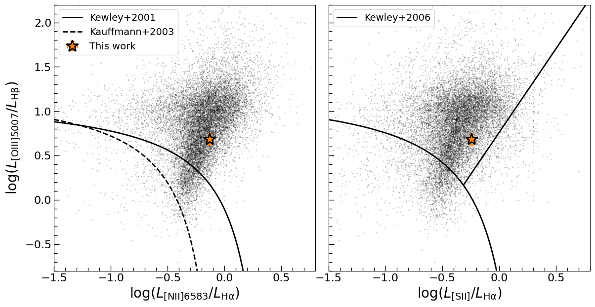
_images/sdss0006_bpt.png — The object against the Liu et al. (2019) AGN sample, on both BPT planes. It sits with the AGN: well above the Kewley et al. (2001) line in the [N II] plane, and on the Seyfert side of the Kewley et al. (2006) line that separates Seyferts from LINERs in the [S II] plane – which is what a 2 900 km/s broad H-alpha and [O III]/H-beta ~ 5 say it should.#

The background points come from Liu2019.fits, which is not in the repository: it is public data (Liu et al. 2019, ApJS 243, 21) and the notebook expects it in develop/temp/. Only the background points need it; the fit does not.

11. The black hole and the host galaxy #

The black-hole mass pairs the two stages, using Liu et al. (2019) Equation 2:

log M_BH = 0.533 log(L_5100 / 1e44) + 2 log(FWHM_Hbeta / 1000) + 6.91

The two posteriors are independent fits, so the two numbers are drawn at random from them and paired; the quoted error is the width that comes out, which now carries both stages. It is not the same as a joint fit’s error – no correlation between the continuum and the line widths can be seen this way – but it is the honest version of what the staged procedure measures.

# %% mbh_sigma
# Table 2 and 3 of Kormendy & Ho (2013, ARA&A, 51, 511)
tb2 = Table.read(TABLE_DIR / 'tab2.ipac', format='ascii.ipac')
tb3 = Table.read(TABLE_DIR / 'tab3.ipac', format='ascii.ipac')

Mbh_k13 = np.concatenate([tb2['Mbh'], tb3['Mbh']])
lMbh_k13 = np.concatenate([tb2['lMbh'], tb3['lMbh']])
uMbh_k13 = np.concatenate([tb2['uMbh'], tb3['uMbh']])
sigma_k13 = np.ma.concatenate([tb2['sigma'], tb3['sigma']])
esigma_k13 = np.ma.concatenate([tb2['esigma'], tb3['esigma']])
flag = np.concatenate([tb2['flag'], tb3['flag']])
flag_ell = np.concatenate([np.ones_like(tb2['Mbh']), np.zeros_like(tb3['Mbh'])])  # 1 for elliptical, 0 for disk

fig, ax = plt.subplots(figsize=(7, 7))

logMbh_med = float(np.median(logMbh))
logMbh_e = np.percentile(logMbh, [16, 84])
ax.errorbar(sigma_star, 10**logMbh_med,
            xerr=[[sigma_star - sigma_star_lo], [sigma_star_hi - sigma_star]],
            yerr=[[10**logMbh_med - 10**logMbh_e[0]], [10**logMbh_e[1] - 10**logMbh_med]],
            ms=20, marker='*', ls='none', color='C1', mec='k', mew=2, label='This work',
            zorder=5, capsize=3)

fltr = (flag == 1) & (flag_ell == 1)
ax.errorbar(sigma_k13[fltr], Mbh_k13[fltr], xerr=esigma_k13[fltr], yerr=[Mbh_k13[fltr] - lMbh_k13[fltr], uMbh_k13[fltr] - Mbh_k13[fltr]],
            fmt='o', ms=5, color='gray', label='Ellipticals')
fltr = (flag == 1) & (flag_ell == 0)
ax.errorbar(sigma_k13[fltr], Mbh_k13[fltr], xerr=esigma_k13[fltr], yerr=[Mbh_k13[fltr] - lMbh_k13[fltr], uMbh_k13[fltr] - Mbh_k13[fltr]],
            fmt='o', ms=5, color='C3', label='Classical bulges')
fltr = (flag == 3)
ax.errorbar(sigma_k13[fltr], Mbh_k13[fltr], xerr=esigma_k13[fltr], yerr=[Mbh_k13[fltr] - lMbh_k13[fltr], uMbh_k13[fltr] - Mbh_k13[fltr]],
            fmt='o', ms=5, color='C0', label='Pseudobulges')
ax.set_xscale('log')
ax.set_yscale('log')
ax.set_xlim([50, 500])
ax.set_ylim([5e5, 2.5e10])

ax.set_xticks([60, 80, 100, 200, 300, 400])
ax.set_xticklabels([60, 80, 100, 200, 300, 400])
ax.set_xlabel(r'$\sigma_e\ (\rm km\ s^{-1})$', fontsize=20)
ax.set_ylabel(r'$M_{\rm BH}\ (M_\odot)$', fontsize=20)
ax.legend(loc='upper left', fontsize=14)
fig.savefig(OUTPUT_DIR / 'sdss0006_mbh_sigma.png', dpi=140, bbox_inches='tight')
plt.show()

print(f"  sigma_* = {sigma_star:.1f} (-{sigma_star - sigma_star_lo:.1f}/+{sigma_star_hi - sigma_star:.1f}) km/s")
print(f"  log M_BH = {logMbh_med:.2f} (-{logMbh_med - logMbh_e[0]:.2f}/+{logMbh_e[1] - logMbh_med:.2f})")

sigma_* = 74.2 (-5.3/+5.6) km/s
log M_BH = 7.10 (-0.17/+0.17)

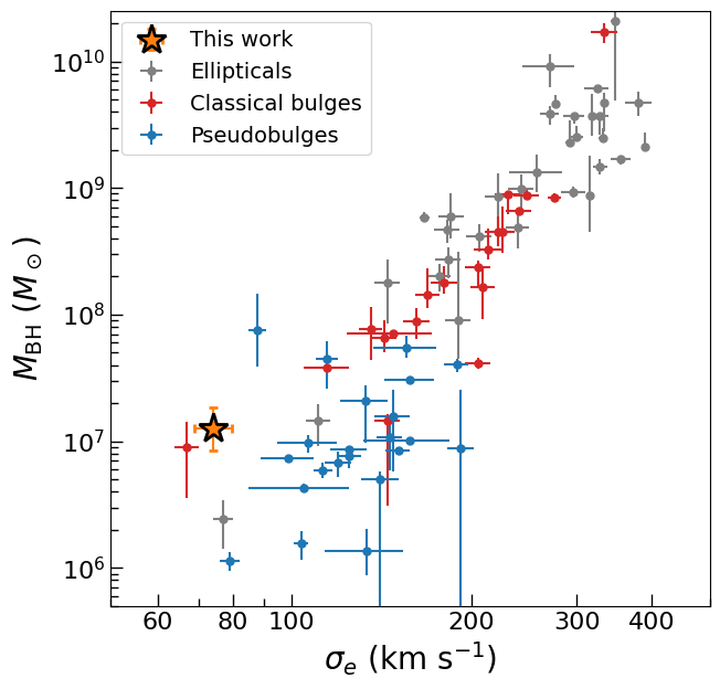
_images/sdss0006_mbh_sigma.png — The object on the M-sigma plane, against the Kormendy & Ho (2013) sample. At `sigma_*` = 74 km/s their relation gives 10^6.8 solar masses; the fit gives 10^7.1, about 0.3 dex above it and inside both its scatter and our own +-0.17 dex. The horizontal error bar is the +-10 km/s of section 5, not the +-5 of the single run.#

12. What the numbers say against the reference fit #

The notebook follows example/wrk_sagan_sdss0006.ipynb – the same windows, the same components, the same atoms – but fits with nested sampling instead of LevMarLSQFitter, so every number comes with a posterior. The comparison is the honest test of the translation:

quantity	reference (LSQ)	this page
sigma_*	79.62 km/s	74.20 (-5.3/+5.6)
lambda L_5100	2.17e42 erg/s	2.27 (-0.28/+0.24)
[S II] template	245 km/s	240 km/s
bHalpha.sigma_c	1102 km/s	1248 (-110/+120)
bHbeta.sigma_c	1240 km/s	1458 (-250/+300)
nHalpha.amplitude	21.09	21.15 (-0.73/+0.73)
[O III] 5007	28.66	30.84 (-1.2/+1.0)
log M_BH	6.95	7.10 (-0.17/+0.17)

Every quantity agrees to within two sigma of the intervals above (the largest gap is [O III] 5007, 1.8 sigma), which is what should happen when the same model is fitted to the same pixels. The differences are largest where the reference’s widths are: broad H-beta is 1 458 here against 1 240, and since the mass goes as its square that is most of the 0.15 dex in log M_BH. That is a real disagreement about the profile’s shape – a least-squares fit pulls the broad H-beta width down towards the narrow feature it overlaps, and it is the sort of thing a posterior makes visible instead of hiding. (The reference notebook prints no mass; its 6.95 is the same equation applied to its own sigma and luminosity.)

13. What to check before believing any of it #

The sampler, first. JNesty defaults to a queue-mode sampler when bound='multi', and on these models that path is not reproducible: repeated runs of the H-alpha stage landed on evidences between -478 and -456 with broad-line widths 40% apart, depending only on how much GPU memory was free when the run started. The notebook sets queue_size=0 (JNesty’s legacy batch mode), under which the same stage reproduces to half a nat and lands where dynesty lands when the same model is written with the astropy classes and sampled on the CPU:

sampler	log Z	sigma(bHalpha)
JNesty, queue off	-460.9	1346 km/s
JNesty, queue off	-461.4	1346 km/s
dynesty (CPU)	-461.8 +- 0.2	1350 (+1212, +1497)

``nlive``, second. 400 live points under-sample the broad-line amplitude-width ridge and the evidence moves by several nats between runs even with the queue off; 2 000 is where the stages above were sampled.

The stages are separate. Each stage samples its own posterior and the next one reads the previous one’s median, not its posterior: the continuum is subtracted at its medians before the [S II] window is fitted, and the [S II] template is frozen when H-alpha is. A joint fit over the whole spectrum would carry every correlation; this is the staged procedure the reference notebook uses, done with posteriors.

The template has the instrumental resolution in it. The [S II] profile includes the SDSS line-spread function, 2.4 A in FWHM – 107 km/s at 6 700 A – so the widths above are observed, not corrected. If the gas kinematics matter, subtract it in quadrature; the reference notebook does not, and neither does this one.

14. Saving the fit, and where to go next #

The last stage is written to a FITS file that load_jnesty_fit_from_fits reads back into a JNesty_Fit: the samples and their weights, the evidence, the parameters, prior bounds and ties, the model description and the spectrum. Everything after the sampler in this page can then be redone without resampling.

# %% save
fits_path = OUTPUT_DIR / 'sdss0006_jax_fit.fits'
save_jnesty_fit_to_fits(fit_hb, fits_path)
print(f"  wrote {fits_path}  ({fits_path.stat().st_size / 1e6:.0f} MB)")
print(f"  read it back with load_jnesty_fit_from_fits({str(fits_path)!r})")
fit_hb.release_device_buffers()

Example: fitting a strong AGN – the same machinery on a luminous AGN, where the continuum is a power law and the hard part is the narrow-line profile instead.
Priors – the prior shapes used above, and how to make one parameter’s prior depend on another’s.
JAX / GPU acceleration – the JAX backend, the batching, and the CPU-versus-GPU comparison.
Fitting From a Configuration File – the same model and sampler driven from a TOML file, for a whole sample.

Example: measure the black hole and the host galaxy

Contents

Example: measure the black hole and the host galaxy#