Examples

This page walks through fitting real ALMA data with galfit-uv using two models: a single free-n Sersic and a Sersic(n=1) + point source decomposition.

Target

GQC J0054-4955 observed in CO(3-2) at z ~ 2.5.

Demo data: The measurement set can be downloaded from: https://drive.google.com/file/d/1TPZQvP-7wc5Kk169Gh6IgiYAUoaug2bb/view?usp=sharing

• 1980 visibility points after time-averaging
• UV range: 5 -- 111 kilo-lambda
• Wavelength: 2.817 mm
• Zero-baseline flux: ~19.2 mJy

Two models are compared:

Model	Components	Free params
Model A	Single Sersic (free n)	7
Model B	Sersic(n=1) + Point source	7 (n fixed)

Step 1: Export Visibilities

Extract averaged visibility data from the measurement set.

from galfit_uv.export import export_vis, save_uvtable

dvis, wle = export_vis('data/GQC_J0054-4955_avg.ms', verbose=True)

print(f"Extracted {len(dvis.u)} visibility points")
print(f"Wavelength: {wle*1e3:.3f} mm")
print(f"uv range: {dvis.uvdist.min()/1e3:.0f} -- {dvis.uvdist.max()/1e3:.0f} klambda")
print(f"Total flux (zero-baseline): {abs(dvis.vis[0])*1e3:.2f} mJy")

# Optionally save a uvplot-compatible table
save_uvtable(dvis.u, dvis.v, dvis.vis, dvis.wgt, 'uv_table.txt', wle=wle)

Output:

Extracted 1980 visibility points
Wavelength: 2.817 mm
uv range: 5 -- 111 klambda
Total flux (zero-baseline): 19.17 mJy

Step 2: Build the Model

Model A — Single Sersic:

from galfit_uv.models import make_model_fn

model_fn, param_info = make_model_fn(['sersic'])
# labels = ['flux', 'Re', 'n', 'incl', 'PA', 'dx', 'dy']

Model B — Sersic(n=1) + Point:

from galfit_uv.models import make_model_fn

model_fn, param_info = make_model_fn(
    ['sersic', 'point'],
    fixed={'sersic:n': 1.0},
)
# labels = ['sersic:flux', 'sersic:Re', 'point:flux', 'incl', 'PA', 'dx', 'dy']

Step 3: Run MCMC

from galfit_uv.fit import fit_mcmc

result = fit_mcmc(
    dvis, model_fn, param_info,
    max_steps=5000,
    burnin=2500,
    nwalk_factor=5,
    outpath='./fit_output',
    seed=42,
)

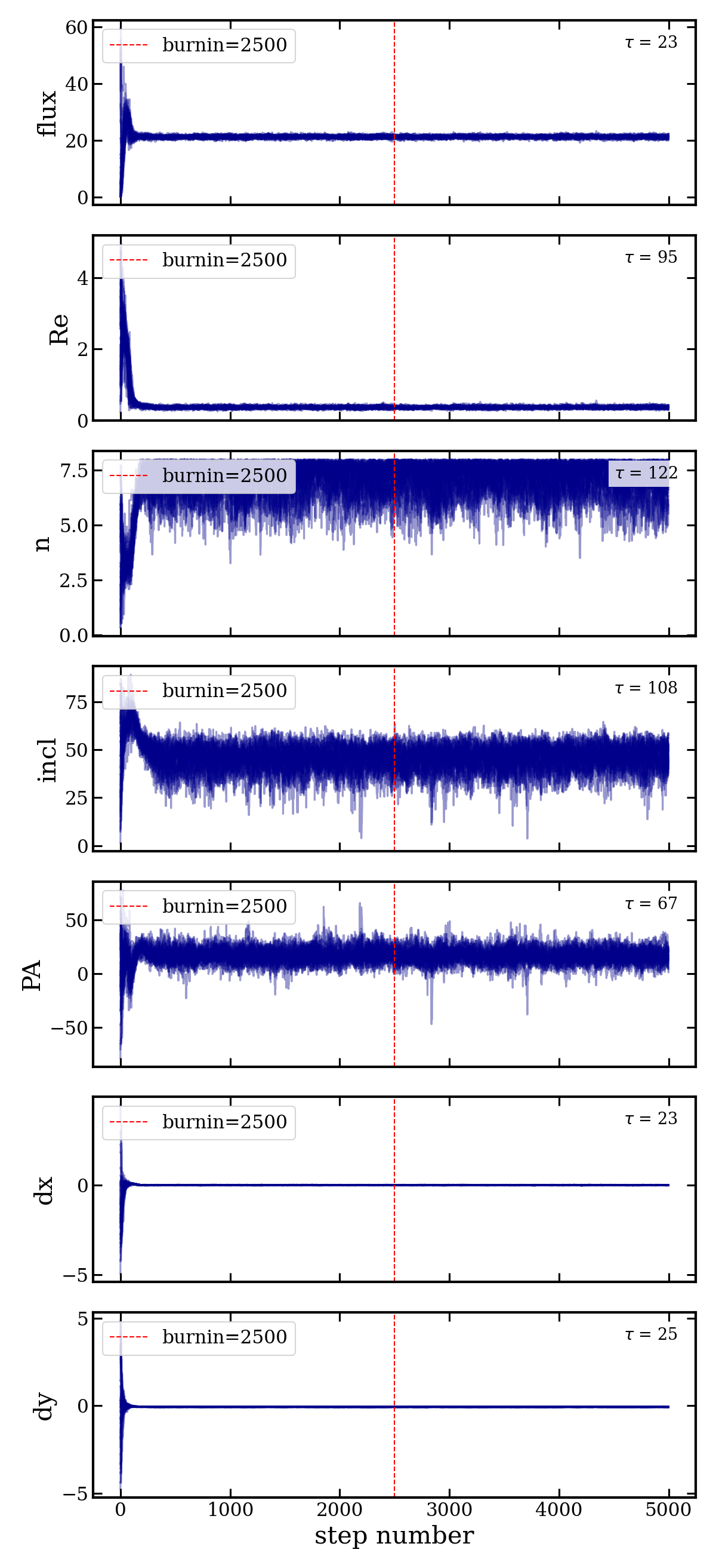
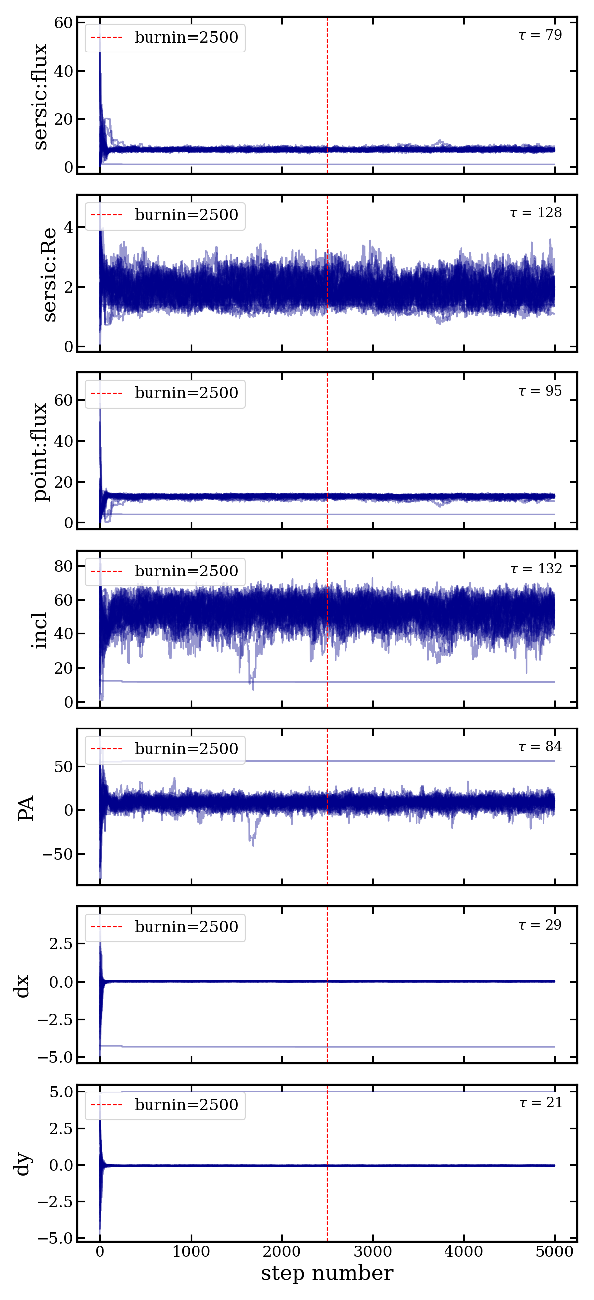
Settings: 35 walkers (7 free params x 5), 5000 steps per walker, 2500 burn-in steps.

Outputs saved to outpath/:

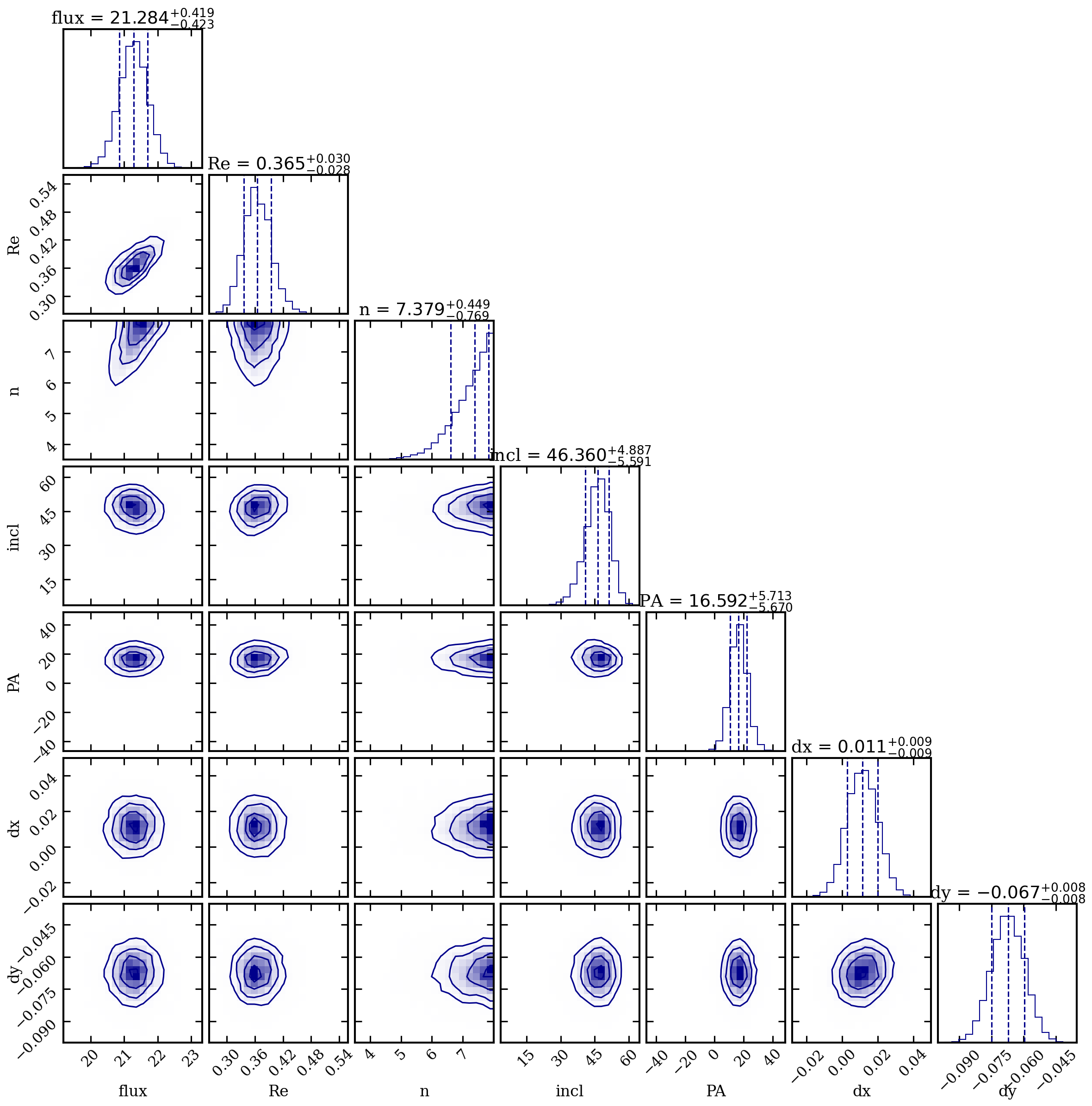
• fit_results.fits — multi-extension FITS with data, model, samples, fit statistics
• chains.png — walker traces with autocorrelation time annotations
• corner_plot.png — posterior corner plot

---

Model A: Single Sersic (free n)

Results

Parameter	Best-fit	+1sig	-1sig
flux (mJy)	21.28	+0.42	-0.42
Re (arcsec)	0.365	+0.03	-0.03
n	7.38	+0.45	-0.77
incl (deg)	46.4	+4.9	-5.6
PA (deg)	16.6	+5.7	-5.7
dx (arcsec)	0.011	+0.009	-0.009
dy (arcsec)	-0.067	+0.008	-0.008

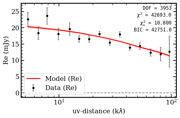
Fit statistics: chi2/DOF = 10.80, BIC = 42751

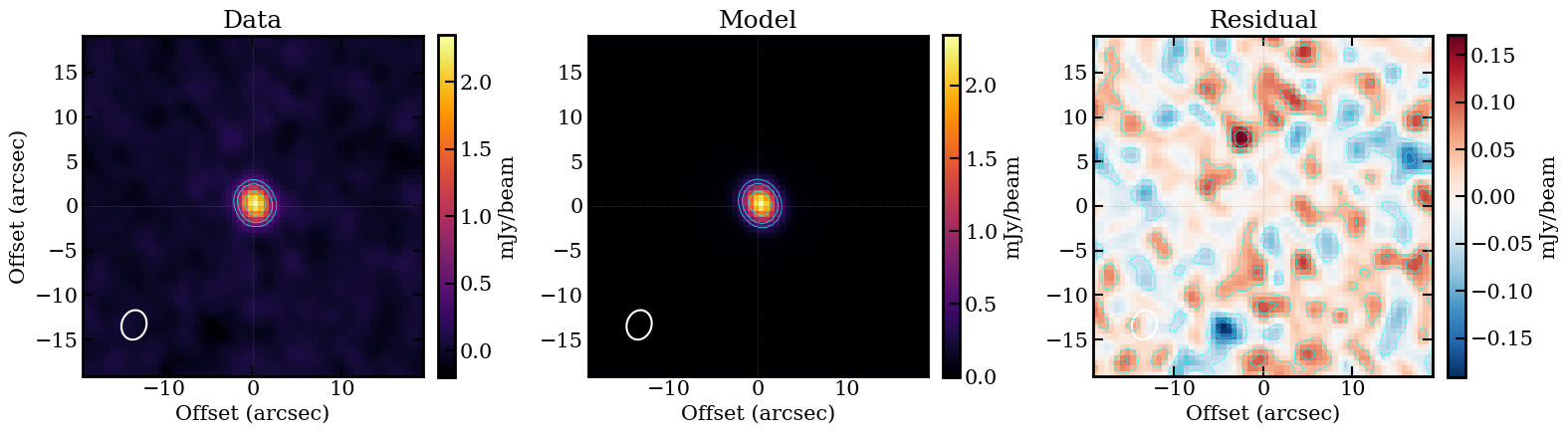
The high Sersic index (n ~ 7.4, well above de Vaucouleurs n=4) indicates a very concentrated core with extended wings, while the small effective radius (Re ~ 0.37 arcsec) is consistent with a compact emission region.

Figures

---

Model B: Sersic(n=1) + Point Source

Results

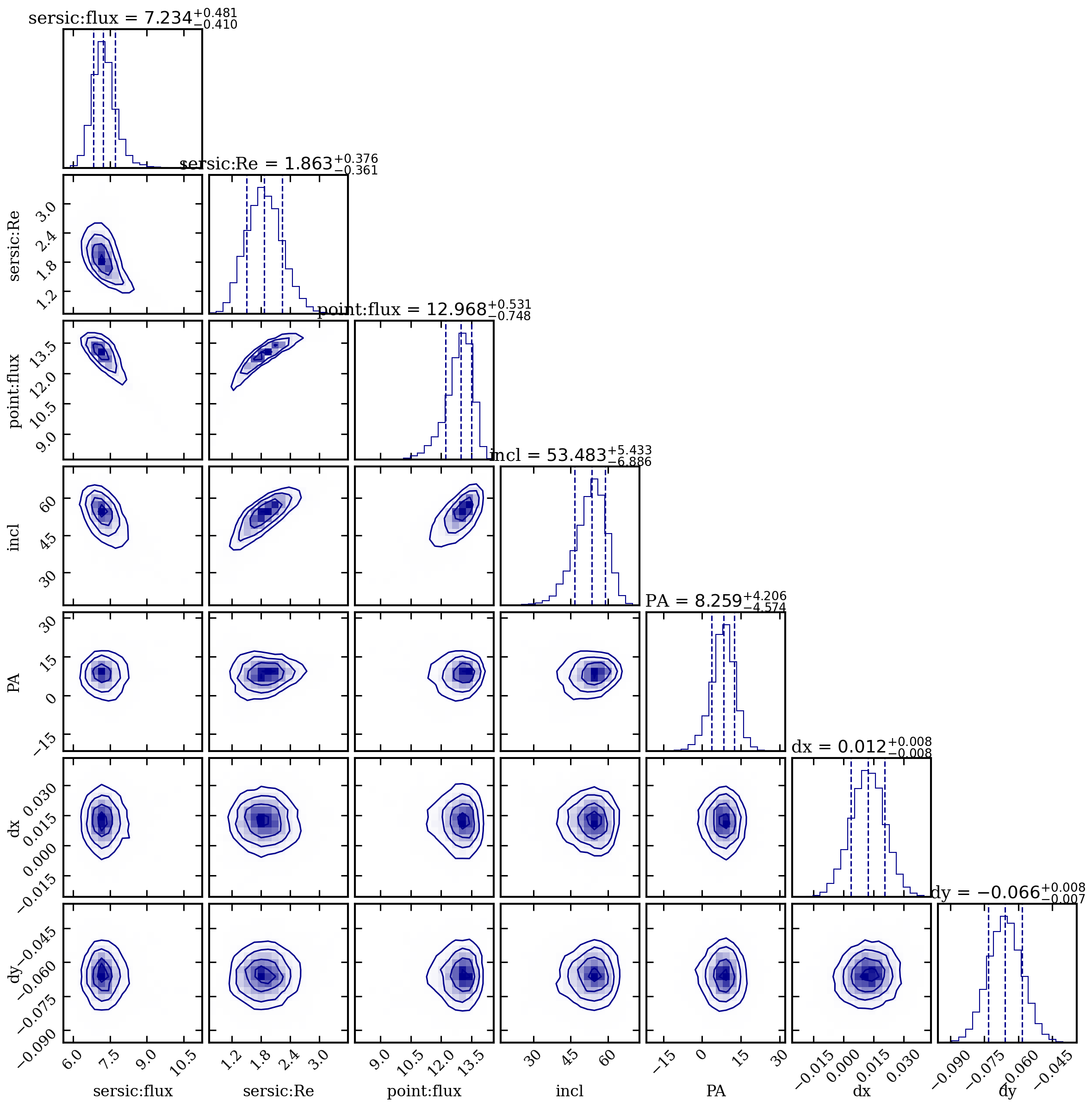
Parameter	Best-fit	+1sig	-1sig
sersic:flux (mJy)	7.23	+0.48	-0.41
sersic:Re (arcsec)	1.86	+0.38	-0.36
sersic:n	1.00	—	— (fixed)
point:flux (mJy)	12.97	+0.53	-0.75
incl (deg)	53.5	+5.4	-6.9
PA (deg)	8.3	+4.2	-4.6
dx (arcsec)	0.012	+0.008	-0.009
dy (arcsec)	-0.066	+0.008	-0.007

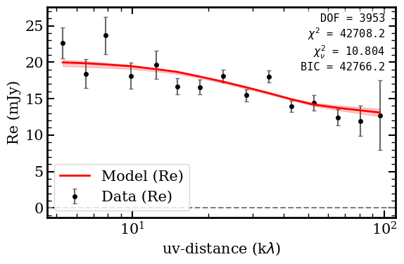
Fit statistics: chi2/DOF = 10.80, BIC = 42766

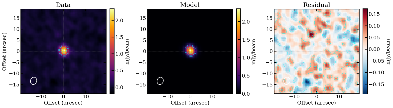
The model decomposes the source into an extended exponential disk (~7.2 mJy, Re ~ 1.86 arcsec) plus a dominant unresolved point source (~13 mJy), with a fitted inclination of ~53 degrees.

Figures

---

Model Comparison

Metric	Model A (Sersic)	Model B (Sersic+Point)
Total flux (mJy)	21.3	7.2 + 13.0 = 20.2
Extended size	Re = 0.37 arcsec	Re = 1.86 arcsec
Sersic index	n = 7.4 (free)	n = 1.0 (fixed)
BIC	42751	42766

Both models yield nearly identical reduced chi-squared values. The single Sersic has a slightly lower BIC, but the two-component decomposition provides a more physically interpretable separation between an extended disk and a compact nucleus. The geometry parameters (center offset) are consistent between the two models.