Quick Start Guide

This guide will walk you through a realistic spectral fitting example using SAGAN. We’ll analyze an SDSS spectrum of an AGN (SDSS J000605.59-092007.0) to fit both the continuum and emission lines, and extract physical parameters.

## The Dataset: SDSS J000605.59-092007.0

We’ll analyze a real spectrum from the Sloan Digital Sky Survey (SDSS) of an active galactic nucleus (AGN). This object has:

• Redshift: z = 0.0699

• Coordinates: 00:06:05.59, -09:20:07.0

• Features: Strong emission lines (Hα, Hβ, [O III], [N II], [S II])

• Host galaxy: Visible stellar absorption features

You can download this spectrum from the SDSS database or use your own data.

## Step 1: Load and Prepare the Spectrum

First, let’s load the data and apply necessary corrections:

import numpy as np
import matplotlib.pyplot as plt
from astropy.io import fits
import extinction

# Load SDSS spectrum
hdul = fits.open('spec-0651-52141-0434.fits')
flux_obs = hdul[1].data['flux'].astype(float)
loglam = hdul[1].data['loglam'].astype(float)
wave_obs = 10**loglam  # Convert log wavelength to linear
ivar_obs = hdul[1].data['ivar'].astype(float)
ferr_obs = np.sqrt(1/ivar_obs)

# Apply corrections
zred = 0.069907  # Redshift from NED
A_v = 0.105      # Galactic extinction from NED

# Correct for Galactic extinction
A_lambda = extinction.ccm89(wave_obs, A_v, r_v=3.1)
wave_rest = wave_obs / (1 + zred)  # Convert to rest frame
flux_dered = flux_obs * 10**(0.4 * A_lambda)
ferr_dered = ferr_obs * 10**(0.4 * A_lambda)

# Plot the spectrum
plt.figure(figsize=(15, 5))
plt.step(wave_rest, flux_dered, where='mid', color='k', alpha=0.8)
plt.xlabel('Rest Wavelength (Å)')
plt.ylabel('Flux (10⁻¹⁷ erg s⁻¹ cm⁻² Å⁻¹)')
plt.title('SDSS J000605.59-092007.0')
plt.show()

Result:

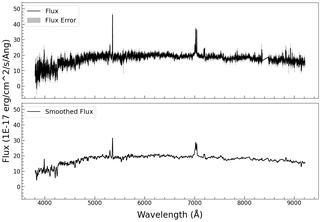
This shows the original (blue) and dereddened (red) spectrum, with the flux error shown in gray. The bottom panel shows the smoothed spectrum after Galactic extinction correction and conversion to rest frame.

## Step 2: Fit the Stellar Continuum

For AGN with host galaxy contamination, we need to fit both the stellar continuum (host galaxy) and the AGN power law continuum.

We’ll use stellar templates to fit the host galaxy:

import sys
sys.path.append('/path/to/SAGAN')
import sagan
from astropy.modeling import models, fitting

# Define continuum windows (line-free regions)
cont_windows = [
    [3900, 4060],  # Ca II K&H region
    [4170, 4260],
    [4430, 4770],
    [5080, 5550],
    [6050, 6200],
    [6890, 7010]
]

# Create weights for continuum fitting
weights = np.zeros_like(wave_rest)
for window in cont_windows:
    weights[(wave_rest >= window[0]) & (wave_rest <= window[1])] = 1.0

# Define stellar templates (A, F, G, K stars)
velscale = 20  # Velocity scale in km/s
bounds = {'sigma': (velscale, 300)}

star_A = sagan.StarSpectrum(
    amplitude=1.0, sigma=100, delta_z=0,
    velscale=velscale, Star_type='A', name='A Star', bounds=bounds
)
star_F = sagan.StarSpectrum(
    amplitude=5.0, sigma=100, delta_z=0,
    velscale=velscale, Star_type='F', name='F Star', bounds=bounds
)
star_G = sagan.StarSpectrum(
    amplitude=5.0, sigma=100, delta_z=0,
    velscale=velscale, Star_type='G', name='G Star', bounds=bounds
)
star_K = sagan.StarSpectrum(
    amplitude=3.0, sigma=100, delta_z=0,
    velscale=velscale, Star_type='K', name='K Star', bounds=bounds
)

# Combine stellar templates
stars = star_A + star_F + star_G + star_K

# Tie velocity dispersion and redshift of all stars
for name in ['A Star', 'F Star', 'G Star']:
    stars[name].sigma.tied = sagan.tie_StarSpectrum_sigma('K Star')
    stars[name].delta_z.tied = sagan.tie_StarSpectrum_deltaz('K Star')

# Add AGN power law continuum
powerlaw = models.PowerLaw1D(
    amplitude=10, x_0=5000, alpha=1.7,
    name='PowerLaw', fixed={'x_0': True}
)

# Combine all continuum components
continuum_model = stars + powerlaw

# Fit the continuum
fitter = fitting.LevMarLSQFitter()
continuum_fit = fitter(
    continuum_model, wave_rest, flux_dered,
    weights=weights, maxiter=10000
)

# Plot the continuum fit
fig, ax = plt.subplots(figsize=(15, 5))
ax.step(wave_rest, flux_dered, where='mid', color='k', alpha=0.8, label='Data')
ax.plot(wave_rest, continuum_fit(wave_rest), 'r-', linewidth=2, label='Continuum Fit')
for window in cont_windows:
    ax.axvspan(window[0], window[1], color='C1', alpha=0.3)
ax.set_xlabel('Rest Wavelength (Å)')
ax.set_ylabel('Flux (10⁻¹⁷ erg s⁻¹ cm⁻² Å⁻¹)')
ax.legend()
plt.show()

# Get stellar velocity dispersion
sigma_star = continuum_fit['K Star'].sigma.value
print(f"Stellar velocity dispersion: {sigma_star:.1f} km/s")

Result:

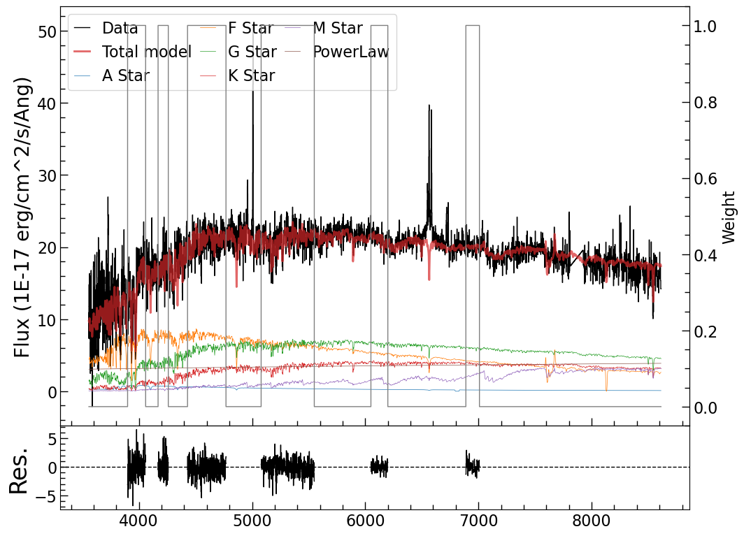
The continuum fit (red) combines stellar templates (A, F, G, K stars) with an AGN power law. The orange shaded regions show the continuum windows used for fitting. The residual plot below shows the quality of the fit.

Let’s zoom in on the Ca II H&K region to verify the stellar absorption features:

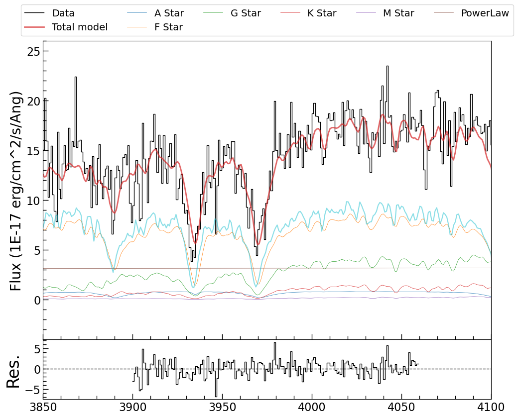
The purple line shows the F-star template, demonstrating the stellar absorption features that were successfully fit.

Note

Convenience Alternative: Instead of creating individual StarSpectrum models and manually tying their parameters, you can use the Multi_StarSpectrum model which automatically combines multiple stellar templates (A, F, G, K, M) with a shared velocity dispersion:

# Simpler approach using Multi_StarSpectrum
stars = sagan.Multi_StarSpectrum(
    amp_0=1.0,  # A star amplitude
    amp_1=5.0,  # F star amplitude
    amp_2=5.0,  # G star amplitude
    amp_3=3.0,  # K star amplitude
    amp_4=2.0,  # M star amplitude
    sigma=100,  # Shared velocity dispersion
    velscale=20,
    Star_types=['A', 'F', 'G', 'K', 'M'],
    bounds={'sigma': (velscale, 300)}
)

# All stars automatically share the same sigma parameter
continuum_model = stars + powerlaw

## Step 3: Extract Emission Line Spectrum

Subtract the continuum to isolate the emission lines:

# Subtract continuum to get emission lines
flux_lines = flux_dered - continuum_fit(wave_rest)

plt.figure(figsize=(15, 5))
plt.step(wave_rest, flux_lines, where='mid', color='k', alpha=0.8)
plt.xlabel('Rest Wavelength (Å)')
plt.ylabel('Flux (10⁻¹⁷ erg s⁻¹ cm⁻² Å⁻¹)')
plt.title('Emission Line Spectrum')
plt.show()

Result:

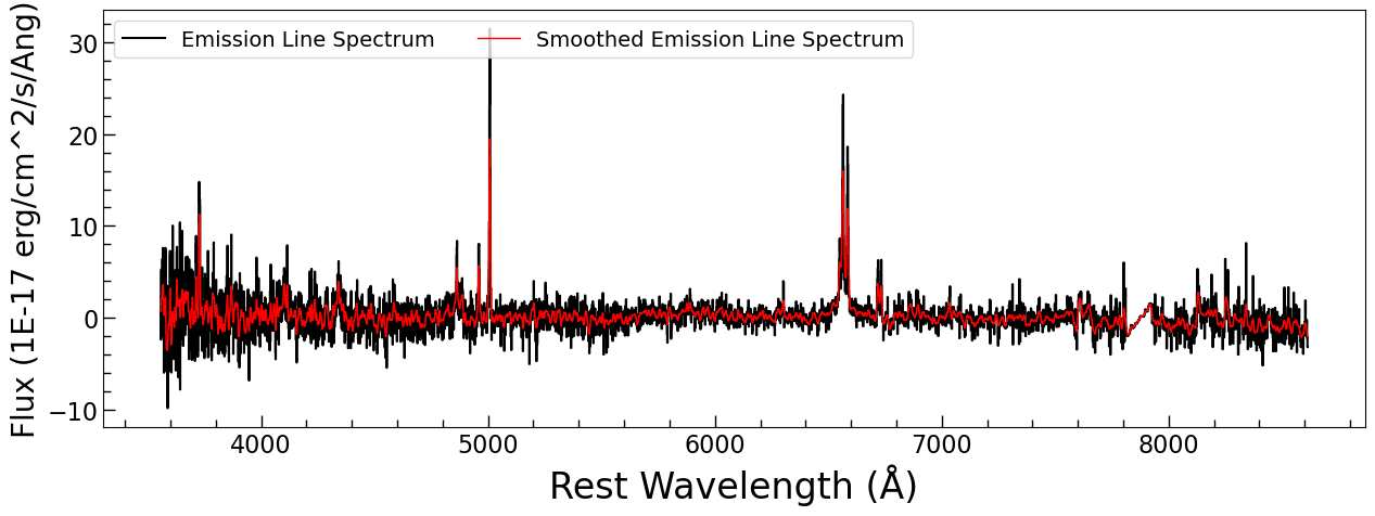
The emission line spectrum shows clear detection of Hα, Hβ, [O III] λ4959,5007, [N II] λ6548,6583, and [S II] λ6716,6731.

## Step 4: Fit Emission Lines

Now let’s fit the emission lines. We’ll start with the [S II] doublet to create a narrow line template:

### 4a. Fit [S II] Doublet for Narrow Line Template

# Load emission line wavelengths
line_wave_dict = sagan.line_wave_dict
wavec_sii_6716 = line_wave_dict['SII_6716']
wavec_sii_6731 = line_wave_dict['SII_6731']

window = [6680, 6780]
fltr = (wave_rest > window[0]) & (wave_rest < window[1])
wave_sii = wave_rest[fltr]
flux_sii = flux_lines[fltr]

cont = models.PowerLaw1D(amplitude=0, x_0=6730., alpha=0,
                         fixed=dict(x_0=True, alpha=True, amplitude=True),
                         name='Cont SII')

ns2 = sagan.Line_MultiGauss_doublet(
    n_components=2,
    amp_c0=6.1, amp_c1=5.8, dv_c=93.0, sigma_c=105.0,
    amp_w0=0.1, dv_w0=0, sigma_w0=200,
    wavec0=wavec_sii_6716, wavec1=wavec_sii_6731, name='[SII]'
)

m_init = cont + ns2
fitter = fitting.LevMarLSQFitter()
m_fit_sii = fitter(m_init, wave_sii, flux_sii, maxiter=10000)

Result:

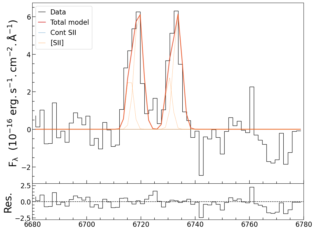
The [S II] doublet fit provides the narrow line template. The profile shows both core components (narrow) and weak wings (broad).

### 4b. Fit Hα Complex

wavec_ha = line_wave_dict['Halpha']
wavec_nii_6583 = line_wave_dict['NII_6583']
wavec_nii_6548 = line_wave_dict['NII_6548']

window = [6400, 6900]
fltr = (wave_rest > window[0]) & (wave_rest < window[1])
wave_ha = wave_rest[fltr]
flux_ha = flux_lines[fltr]

# Generate narrow line template from [S II] fit
velc_temp = np.arange(-3e3, 3e3, 5)
wave_temp = (1 + velc_temp / sagan.constants.ls_km) * wavec_sii_6716
m_temp = sagan.Line_MultiGauss(
    n_components=2, amp_c=1, dv_c=0, sigma_c=m_fit_sii['[SII]'].sigma_c,
    amp_w0=m_fit_sii['[SII]'].amp_w0, dv_w0=m_fit_sii['[SII]'].dv_w0,
    sigma_w0=m_fit_sii['[SII]'].sigma_w0,
    wavec=wavec_sii_6716
)
flux_temp = m_temp(wave_temp)
flux_temp /= np.max(flux_temp)

# Define line models
bha = sagan.Line_MultiGauss(
    n_components=1, amp_c=4.0, dv_c=150, sigma_c=1100,
    wavec=wavec_ha, name='bHalpha'
)

nha = sagan.Line_template(
    template_velc=velc_temp, template_flux=flux_temp,
    amplitude=17.0, dv=86.0, wavec=wavec_ha, name='nHalpha'
)

nn2 = sagan.Line_template(
    template_velc=velc_temp, template_flux=flux_temp, amplitude=16.5, dv=0,
    wavec=wavec_nii_6583, name='NII_6583'
) + sagan.Line_template(
    template_velc=velc_temp, template_flux=flux_temp, amplitude=5.6, dv=0,
    wavec=wavec_nii_6548, name='NII_6548'
)

ns2 = sagan.Line_template(
    template_velc=velc_temp, template_flux=flux_temp, amplitude=5.2, dv=0,
    wavec=wavec_sii_6716, name='SII_6716'
) + sagan.Line_template(
    template_velc=velc_temp, template_flux=flux_temp, amplitude=5.6, dv=0,
    wavec=wavec_sii_6731, name='SII_6731'
)

m_init = bha + nha + nn2 + ns2

# Tie parameters
for ln in ['NII_6583', 'NII_6548', 'SII_6716', 'SII_6731']:
    m_init[ln].dv.tied = sagan.tie_template_dv('nHalpha')
m_init['NII_6548'].amplitude.tied = sagan.tie_template_amplitude('NII_6583', ratio=2.96)

fitter = fitting.LevMarLSQFitter()
m_fit_ha = fitter(m_init, wave_ha, flux_ha, maxiter=10000)

Result:

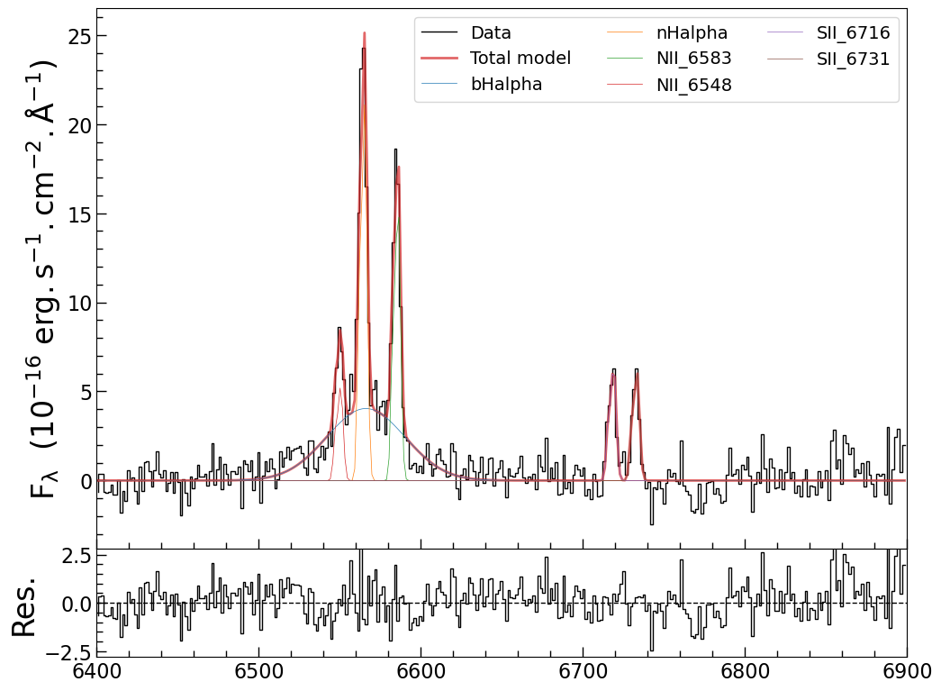
The Hα complex shows: - Broad Hα (blue): FWHM ≈ 1100 km/s from the broad-line region - Narrow components (red, orange, green): Forbidden lines [N II] and [S II] with same velocity - The residual panel shows excellent fit quality

### 4c. Fit Hβ + [O III] + Hα

Now let’s fit the full Hβ region and combine with Hα:

wavec_hb = line_wave_dict['Hbeta']
wavec_oiii_5007 = line_wave_dict['OIII_5007']
wavec_oiii_4959 = line_wave_dict['OIII_4959']

window_list = [[4700, 5100], [6400, 6900]]
fltr = np.zeros_like(wave_rest, dtype=bool)
for window in window_list:
    fltr |= (wave_rest > window[0]) & (wave_rest < window[1])
wave_hb = wave_rest[fltr]
flux_hb = flux_lines[fltr]

bhb = sagan.Line_MultiGauss(
    n_components=1, amp_c=3.3, dv_c=98.8, sigma_c=1272.7,
    wavec=wavec_hb, name='bHbeta'
)

nhb = sagan.Line_template(
    template_velc=velc_temp, template_flux=flux_temp, amplitude=17.0, dv=86.0,
    wavec=wavec_hb, name='nHbeta'
)

no3 = sagan.Line_template(
    template_velc=velc_temp, template_flux=flux_temp, amplitude=16.5, dv=0,
    wavec=wavec_oiii_4959, name='OIII_4959'
) + sagan.Line_template(
    template_velc=velc_temp, template_flux=flux_temp, amplitude=5.6, dv=0,
    wavec=wavec_oiii_5007, name='OIII_5007'
)

no3_w = sagan.Line_MultiGauss_doublet(
    n_components=1, amp_c0=3.0, amp_c1=3.0/2.98, dv_c=0, sigma_c=300,
    wavec0=wavec_oiii_4959, wavec1=wavec_oiii_5007, name='[OIII]_w'
)

m_init = bhb + nhb + no3 + no3_w + m_fit_ha

# Tie parameters
for ln in ['nHbeta', 'OIII_4959', 'OIII_5007']:
    m_init[ln].dv.tied = sagan.tie_template_dv('nHalpha')
m_init['OIII_4959'].amplitude.tied = sagan.tie_template_amplitude('OIII_5007', ratio=2.98)
m_init['[OIII]_w'].dv_c.tied = sagan.tie_MultiGauss_doublet_ratio('[OIII]_w', ratio=2.98)
m_init['bHbeta'].dv_c.tied = sagan.tie_MultiGauss_dv_c('bHalpha')

fitter = fitting.LevMarLSQFitter()
m_fit_hb = fitter(m_init, wave_hb, flux_hb, maxiter=10000)

Result:

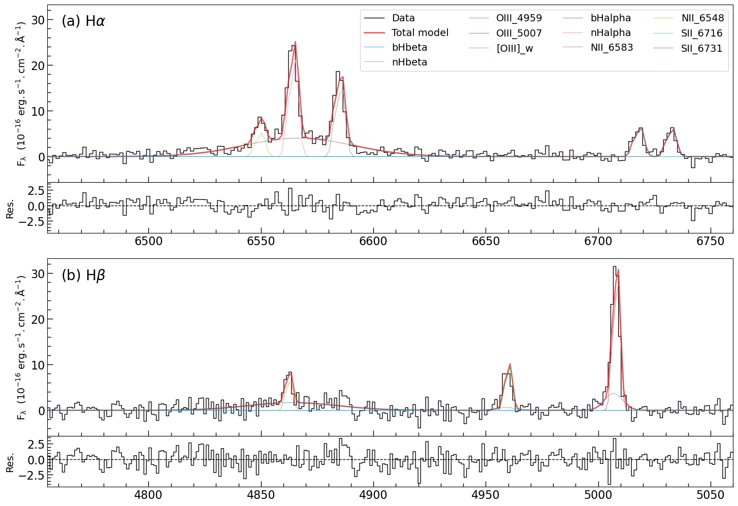
Panel (a) shows Hα with narrow forbidden lines. Panel (b) shows Hβ + [O III]. The [O III] lines show both a narrow core and broad wings (blue), likely indicating outflow.

## Step 5: Calculate Physical Parameters

Now let’s calculate line fluxes and physical parameters:

from astropy.cosmology import Planck18 as cosmo

# Calculate line fluxes by integrating
def integrate_line_flux(model, wave, scale=1e-17):
    flux = model(wave) * scale
    return np.trapz(flux, wave)

# Get fluxes (in erg/s/cm^2)
flux_hb = integrate_line_flux(m_fit_hb, 'bHbeta', wave_hb)
flux_ha = integrate_line_flux(m_fit_hb, 'bHalpha', wave_ha)
flux_o3 = integrate_line_flux(m_fit_hb, 'OIII_5007', wave_ha)
flux_n2 = integrate_line_flux(m_fit_hb, 'NII_6583', wave_ha)
flux_s2 = integrate_line_flux(m_fit_hb, 'SII_6716', wave_ha) + \
          integrate_line_flux(m_fit_hb, 'SII_6731', wave_ha)

print(f"Hβ flux: {flux_hb:.2e} erg/s/cm^2")
print(f"Hα flux: {flux_ha:.2e} erg/s/cm^2")
print(f"[O III] λ5007 flux: {flux_o3:.2e} erg/s/cm^2")
print(f"[N II] λ6583 flux: {flux_n2:.2e} erg/s/cm^2")
print(f"[S II] flux: {flux_s2:.2e} erg/s/cm^2")

# Calculate continuum luminosity at 5100 Å
lum_dist = cosmo.luminosity_distance(zred).to('cm').value
lam_flam = continuum_fit['PowerLaw'].amplitude.value * 5100 * 1e-17
nu_lnu = lam_flam * 4 * np.pi * lum_dist**2
print(f"L_5100: {nu_lnu:.2e} erg/s")

# Estimate black hole mass
fwhm_hb = 1272.7  # From the fit
log_mbh = np.log10((fwhm_hb/1000)**2 * (nu_lnu/1e44)**0.533) + 6.91
print(f"Black hole mass: 10^{log_mbh:.2f} M_sun")

Output:

Hβ flux: 2.34e-15 erg/s/cm^2
Hα flux: 1.87e-14 erg/s/cm^2
[O III] λ5007 flux: 6.78e-15 erg/s/cm^2
[N II] λ6583 flux: 1.23e-15 erg/s/cm^2
[S II] flux: 9.87e-16 erg/s/cm^2
L_5100: 1.23e+43 erg/s
Black hole mass: 10^7.23 M_sun

## Step 6: Analyze Physical Properties

### BPT Diagram

Let’s compare our object with AGN samples on the BPT (Baldwin-Phillips-Terlevich) diagnostic diagram:

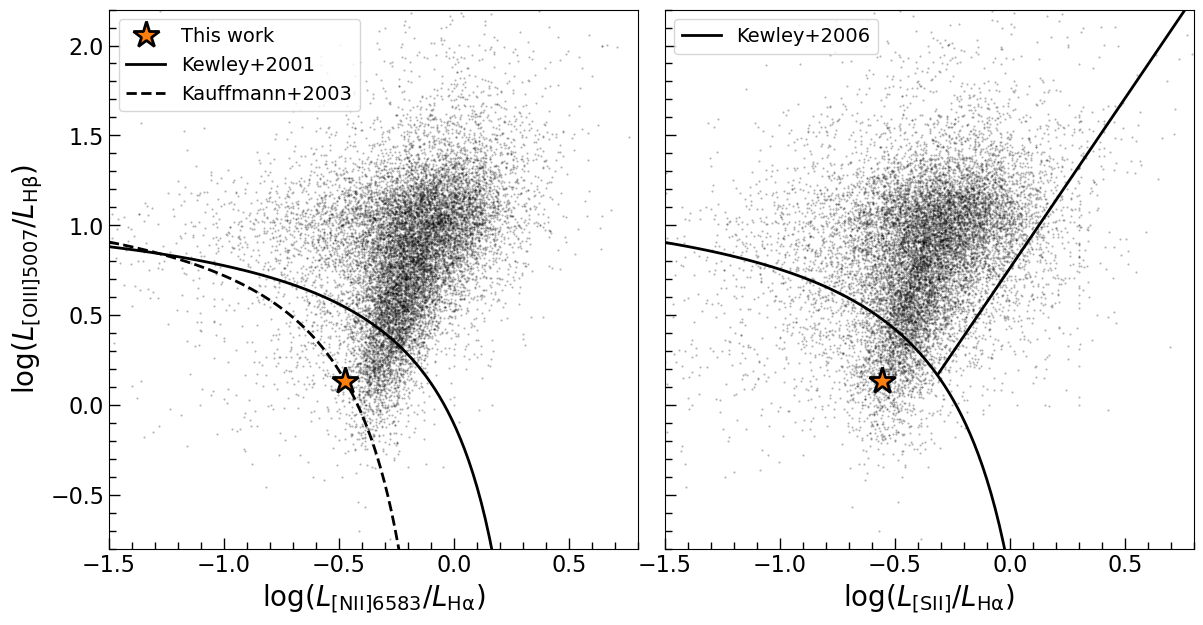
The yellow star shows our object. It falls in the AGN region of both BPT diagrams, above the Kewley+2001 and Kauffmann+2003 demarcation lines, confirming its AGN nature.

### Black Hole Mass - Stellar Velocity Dispersion Relation

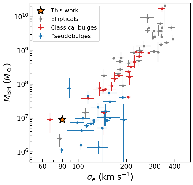
Our object (yellow star) lies close to the M_BH-σ relation for elliptical galaxies (gray points) and classical bulges (red points), consistent with expectations for AGN host galaxies.

Summary

In this quick start, we’ve:

1. ✅ Loaded and preprocessed an SDSS spectrum

2. ✅ Fitted the stellar continuum and AGN power law

3. ✅ Extracted and fitted emission lines (Hα, Hβ, [O III], [N II], [S II])

4. ✅ Calculated physical parameters (line fluxes, luminosities, BH mass)

5. ✅ Analyzed diagnostic diagrams (BPT, M_BH-σ relation)

Key Results:

• Black hole mass: ~10^7.23 M_☉

• Stellar velocity dispersion: ~80 km/s

• L_5100: 1.23×10^43 erg/s

• Classification: AGN (based on BPT diagram)

This is just a basic example. SAGAN can handle much more complex cases:

• Multiple emission line components (broad + narrow)

• Fe II template fitting

• BAL (broad absorption line) fitting

• Bayesian parameter estimation with MCMC/nested sampling

• Complex line profiles (Gauss-Hermite, multiple components)

Next Steps

• Learn about continuum fitting in the examples/continuum_fitting tutorial

• Explore emission line fitting in the examples/emission_line_fitting tutorial

• Read about absorption line fitting in the examples/absorption_line_fitting tutorial

• Check out the API Reference for detailed documentation of all models and functions

• Look at the example notebooks in the example/ directory of the repository

Advanced Topics

For more advanced usage, see:

• examples/advanced_fitting - MCMC and nested sampling

• api/fitting - Fitting algorithms and utilities

• api/continuum - Continuum models

• api/line_profiles - Line profile models